In Figure H, three dye compounds are represented by three peaks separated in time in the chromatogram. Each elutes at a specific location, measured by the elapsed time between the moment of injection [time zero] and the time when the peak maximum elutes. By comparing each peak’s retention time [tR] with that of injected reference standards in the same chromatographic system [same mobile and stationary phase], a chromatographer may be able to identify each compound.
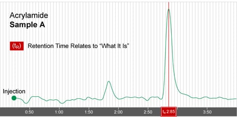
Figure I-1: Identification
In the chromatogram shown in Figure I-1, the chromatographer knew that, under these LC system conditions, the analyte, acrylamide, would be separated and elute from the column at 2.85 minutes [retention time]. Whenever a new sample, which happened to contain acrylamide, was injected into the LC system under the same conditions, a peak would be present at 2.85 minutes [see Sample B in Figure I-2].
[For a better understanding of why some compounds move more slowly [are better retained] than others, please review the HPLC Separation Modes section on page 28].
Once identity is established, the next piece of important information is how much of each compound was present in the sample. The chromatogram and the related data from the detector help us calculate the concentration of each compound. The detector basically responds to the concentration of the compound band as it passes through the flow cell. The more concentrated it is, the stronger the signal; this is seen as a greater peak height above the baseline.
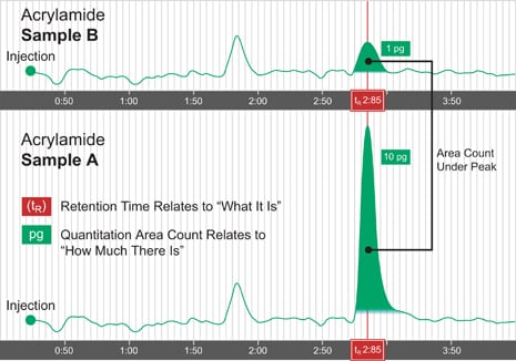
Figure I-2: Identification and Quantitation
In Figure I-2, chromatograms for Samples A and B, on the same time scale, are stacked one above the other. The same volume of sample was injected in both runs. Both chromatograms display a peak at a retention time [tR] of 2.85 minutes, indicating that each sample contains acrylamide. However, Sample A displays a much bigger peak for acrylamide. The area under a peak [peak area count] is a measure of the concentration of the compound it represents. This area value is integrated and calculated automatically by the computer data station. In this example, the peak for acrylamide in Sample A has 10 times the area of that for Sample B. Using reference standards, it can be determined that Sample A contains 10 picograms of acrylamide, which is ten times the amount in Sample B [1 picogram]. Note there is another peak [not identified] that elutes at 1.8 minutes in both samples. Since the area counts for this peak in both samples are about the same, this unknown compound may have the same concentration in both samples.
Isocratic and Gradient LC System Operation
Two basic elution modes are used in HPLC. The first is called isocratic elution. In this mode, the mobile phase, either a pure solvent or a mixture, remains the same throughout the run. A typical system is outlined in Figure J-1.
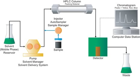
Figure J-1: Isocratic LC System
The second type is called gradient elution, wherein, as its name implies, the mobile phase composition changes during the separation. This mode is useful for samples that contain compounds that span a wide range of chromatographic polarity [see section on HPLC Separation Modes]. As the separation proceeds, the elution strength of the mobile phase is increased to elute the more strongly retained sample components.
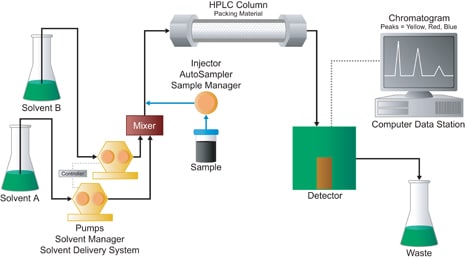
Figure J-2: High-Pressure-Gradient System
In the simplest case, shown in Figure J-2, there are two bottles of solvents and two pumps. The speed of each pump is managed by the gradient controller to deliver more or less of each solvent over the course of the separation. The two streams are combined in the mixer to create the actual mobile phase composition that is delivered to the column over time. At the beginning, the mobile phase contains a higher proportion of the weaker solvent [Solvent A]. Over time, the proportion of the stronger solvent [Solvent B] is increased, according to a predetermined timetable. Note that in Figure J-2, the mixer is downstream of the pumps; thus the gradient is created under high pressure. Other HPLC systems are designed to mix multiple streams of solvents under low pressure, ahead of a single pump. A gradient proportioning valve selects from the four solvent bottles, changing the strength of the mobile phase over time [see Figure J-3].
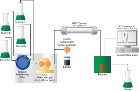
Figure J-3: Low-Pressure-Gradient System
HPLC Scale [Analytical, Preparative, and Process]
We have discussed how HPLC provides analytical data that can be used both to identify and to quantify compounds present in a sample. However, HPLC can also be used to purify and collect desired amounts of each compound, using a fraction collector downstream of the detector flow cell. This process is called preparative chromatography [see Figure K].
In preparative chromatography, the scientist is able to collect the individual analytes as they elute from the column [e.g., in this example: yellow, then red, then blue].
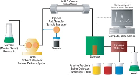
Figure K: HPLC System for Purification: Preparative Chromatography
The fraction collector selectively collects the eluate that now contains a purified analyte, for a specified length of time. The vessels are moved so that each collects only a single analyte peak.
A scientist determines goals for purity level and amount. Coupled with knowledge of the complexity of the sample and the nature and concentration of the desired analytes relative to that of the matrix constituents, these goals, in turn, determine the amount of sample that needs to be processed and the required capacity of the HPLC system. In general, as the sample size increases, the size of the HPLC column will become larger and the pump will need higher volume-flow-rate capacity. Determining the capacity of an HPLC system is called selecting the HPLC scale. Table A lists various HPLC scales and their chromatographic objectives.
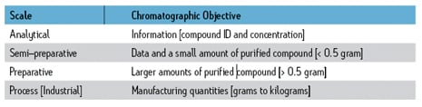
Table A: Chromatography Scale
The ability to maximize selectivity with a specific combination of HPLC stationary and mobile phases—achieving the largest possible separation between two sample components of interest—is critical in determining the requirements for scaling up a separation [see discussion on HPLC Separation Modes]. Capacity then becomes a matter of scaling the column volume [Vc] to the amount of sample to be injected and choosing an appropriate particle size [determines pressure and efficiency; see discussion of Separation Power]. Column volume, a function of bed length [L] and internal diameter [i.d.], determines the amount of packing material [particles] that can be contained (see Figure L).
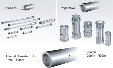
Figure L: HPLC Column Dimensions
In general, HPLC columns range from 20 mm to 500 mm in length [L] and 1 mm to 100 mm in internal diameter [i.d.]. As the scale of chromatography increases, so do column dimensions, especially the cross-sectional area. To optimize throughput, mobile phase flow rates must increase in proportion to cross-sectional area. If a smaller particle size is desirable for more separation power, pumps must then be designed to sustain higher mobile-phase-volume flow rates at high backpressure. Table B presents some simple guidelines on selecting the column i.d. and particle size range recommended for each scale of chromatography.
For example, a semi-preparative-scale application [red X] would use a column with an internal diameter of 10–40 mm containing 5–15 micron particles. Column length could then be calculated based on how much purified compound needs to be processed during each run and on how much separation power is required.
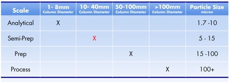
Table B: Chromatography Scale vs. Column Diameter and Particle Size