Method Development Considerations

METHOD DEVELOPMENT CONSIDERATIONS
Column Selection
Ideally, using one column chemistry for all samples, including ordinary peptides (with a mixture of acidic, basic, and non-polar residues), basic peptides, large peptides (30-40 residues), and hydrophobic peptides, reduces the column inventory and eliminates the need to screen multiple columns for each crude sample. While C18 phases are typically used for many peptide separations, the base particle to which the C18 is bonded is also a critical factor that influences chromatographic retention, resolution, and peak shape. XBridge Peptide BEH Columns are based on ethylene bridged hybrid particles rather than pure silica. The BEH (Bridged Ethylsiloxane/Silica Hybrid) particle (Figure 7) minimizes secondary interactions with peptides and is stable at both high and low pH for maximum flexibility in developing separations. The synthetic packing material is available with 130Å or 300Å pores in 3.5, 5, and 10 µm particle sizes. For atypical samples or extremely hydrophobic peptides, the same base particle is available with C8 or C4 bonded phases.

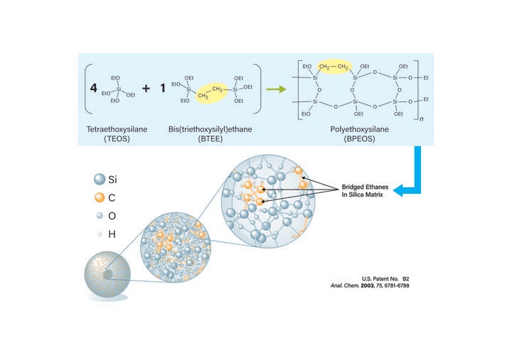
Figure 7: Synthesis of BEH Technology Packing Material.
Approximate peptide mass loading capacities on various column dimensions are shown in Table 1.

Table 1: Approximate Peptide Mass Loading Capacity for Reversed Phase Chromatography (total load in mg).
*5 µm and 10 µm OBD™ Prep Columns; ** 10 µm OBD Prep Columns.
Many factors affect the mass capacity of preparative columns. The listed capacities represent an “average” estimate with reasonable flow rates and injection volumes for each dimension. The following factors are worthy of consideration:
1) Capacity for peptides depends primarily on solubility of the particular sample.
2) Capacity is lower where higher resolution is required.
3) Capacity is dependent on loading conditions, but less so than for small molecules.
a) Peptides are usually loaded in highly aqueous conditions, often with the addition of TFA. Volume loading capacity under these conditions is virtually unlimited. Capacity is limited by solubility during elution.
b) Dried peptides may be wetted with solvents like DMF or DMSO. They are often then diluted with water containing TFA, as above.
c) In some cases, peptides will be dissolved in DMF or DMSO and injected in that solution. The volume guidelines in the chart apply to this condition.
4) Reasonable injection volumes are based on column diameter at a length of 50 mm with relatively strong solvents. Increased length is compatible with larger injection volume, but not proportionately. Weaker solvents significantly increase injection volume.
5) Reasonable flow rates are based on column diameter. Systems will be limited by increasing backpressure with increasing length and decreasing particle size. Some users prefer to run peptides more slowly than small molecules, so would use half the suggested flow rate but with double the gradient duration.
The suitability of the XBridge Peptide BEH C18 130Å as the column of choice for standard peptide isolations was defined by the results obtained after testing a panel of four peptides with different properties. The peptide sequences are proprietary, but notable properties of each peptide are listed in Table 2.

Table 2: Peptide Test Panel Properties.
Peptides are amphiprotic, due to the presence of both weakly acidic (carboxylic acid) and weakly basic (amino) functional groups. Because peptides have both positive and negative charges, they are called zwitterions. If a peptide is subjected to an electric field when dissolved in a solution with a specific hydrogen ion concentration and it does not migrate, that hydrogen ion concentration is the isoelectric point (pI) for the peptide.13, 14, 15 To simplify, therefore, the isoelectric point (pI) is the pH at which the peptide has zero net charge.
As described by Browne, Bennet, and Solomon1,6 HPLC index predicts the percentage of acetonitrile required to elute the peptide from a C18 µBondapak® Column using TFA:water:acetonitrile as the buffer system. They isolated peptides from biological matices and predicted the elution profile based on amino acid composition. High HPLC index values, therefore, suggest increased hydrophobicity on a C18 column. The values will change, obviously, with different columns and mobile-phases, but this straightforward system provides some predictive information about the nature of the peptides.
The chromatographic profiles of the four peptides in the test panel, under very common conditions – 0.1% formic acid in water and in acetonitrile with a gradient from 5-50%B in 50 minutes, is shown in Figure 8. All four model peptides show perfectly acceptable chromatography with sharp, symmetrical peaks.

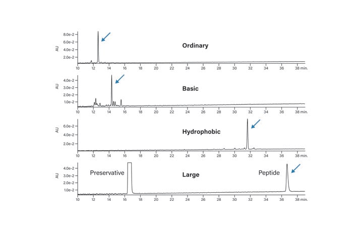
Figure 8: Separation of test peptides under standard conditions.
It is important to consider whether there would be any chromatographic improvement for the large or hydrophobic peptides by using a 300Å pore size column. The largest peptide in the peptide test panel, with 39 residues and a molecular weight over 4000 Da, shows little improvement in peak shape with the larger pore size packing material (Figure 9). The peptide elutes slightly earlier, with the difference being equivalent to about 1-2% acetonitrile. There will be some size limit on using the 130Å pore size packing material. It is most likely above approximately 40 residues.

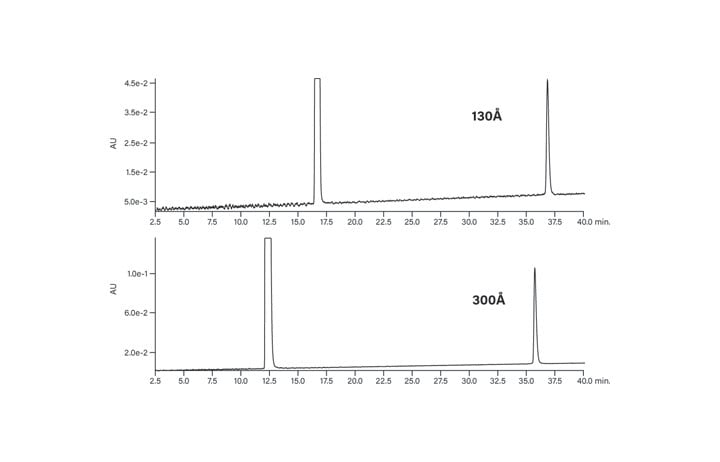
Figure 9: Effect of pore size on the chromatography of the large peptide.
The hydrophobic peptide, with an HPLC index of 113, also elutes as a sharp, symmetrical peak on both the 130Å and 300Å packings (Figure 10). Peptide conformation, the way the peptide is folded in solution, may also influence the best choice of pore size for a particular separation. Just as there are no hard and fast rules for peptide loading capacity, individual peptide properties will also play a role in deciding the best pore size to use. From the experiments discussed above, it can be suggested that the XBridge Peptide BEH Columns, with C18 bonded phase and 130Å pores are ¬a reasonable choice as a starting point for peptide isolation.

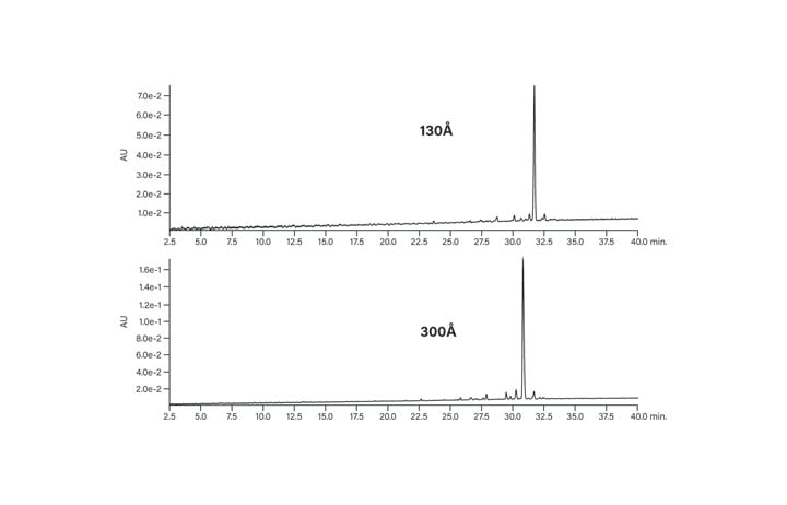
Figure 10: Effect of pore size on the chromatography of the hydrophobic peptide.
From the standpoint of economics and efficiency in performing peptide isolation at the larger scale, it is important to consider particle size. The basic peptide, run on three different particle size columns, illustrates the consistency of the separation (Figure 11). Although the peaks are wider and less well-resolved with the larger particle size, for scalable BEH column packings, the chemical selectivity is unchanged whether the particle size is 3.5, 5, or 10 µm. Large scale isolations benefit from increased particle size, permitting faster flow rates on increasingly wider diameter columns with manageable pressure limits, all of which improve loading capacity, reduce the number of chromatographic runs, and save time and resources.

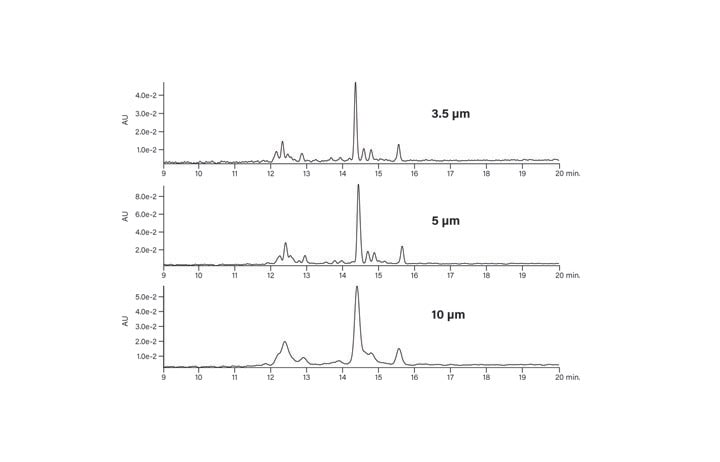
Figure 11: Effect of particle size on the chromatography of the basic peptide.
Although peptides have unique properties that influence the success of their isolation from crude mixtures, the basic principles of prep chromatography17, 18 still apply. While the standard peptide isolation protocol with a generic gradient (such as 5-50%B or 5-95%B) on a reversed-phase column can be used much of the time, peptides with unique properties sometimes need separation method development to realize purity, loading, or yield requirements. Separation methods can often be improved by changing mobile-phase solvent, modifier, gradient slope, temperature, pH, or sample introduction method. Each of these factors impacts the separation, the quality of the chromatography, and the ultimate success of the isolation.

Role of Solvent
The mobile-phase is comprised of three components, the weak solvent, the strong solvent, and the modifier. In reversed-phase chromatography, the weak solvent is almost always water. Although methanol, ethanol, or isopropanol may be considered for fulfilling the role of strong solvent, acetonitrile is usually the solvent of choice because of its low viscosity, slightly higher solvent strength, and its usability in the low wavelength UV detection range (185-205 nm)1.9 Acetonitrile usually provides the best peak shape, is easy to evaporate, and reduces the number of side reactions that can proceed during isolation and workup. Good UV transparency gives high signal to noise for better peak detection. Some users, however, may object to the use of acetonitrile if they want to use the peptide in biological testing. Substituting an alcohol, such as ethanol, reduces the residual toxicity that may be associated with acetonitrile. In addition to concerns about biocompatibility, propanol or acetonitrile:propanol mixtures often increase the solubility of large or hydrophobic peptides and break up aggregates that sometimes form in solution. The effect of 70% isopropanol: 30% acetonitrile on the basic peptide is shown in Figure 12. The resolution of the main peak is improved with respect to its most closely-eluting contaminants and the retention time is reduced by about half. Elevated column temperatures are typically required with mobile-phases containing alcohols due to their higher viscosity.

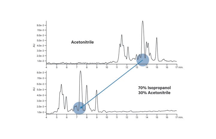
Figure 12: Effect of solvent on the elution of the basic peptide.

Role of Mobile-Phase Modifier
Peptide isolation using reversed-phase chromatography requires the addition of a polar modifier to the mobile-phase since peptides have both positive (amino terminus) and negative (carboxyl terminus) charges that reduce affinity for the hydrophobic surface of the packing material. The side chain protecting groups may also carry a charge, as shown in Figure 13. Modifiers control the pH to change the degree of ionization of the weakly acidic or basic side chains. The modifier may also form ion pairs with the peptide. The separation of a particular sample may be optimized by manipulating these mechanisms.

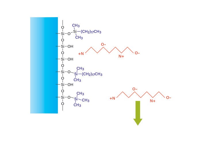
Figure 13: Reversed-phase peptide retention in an aqueous solution without modifier.

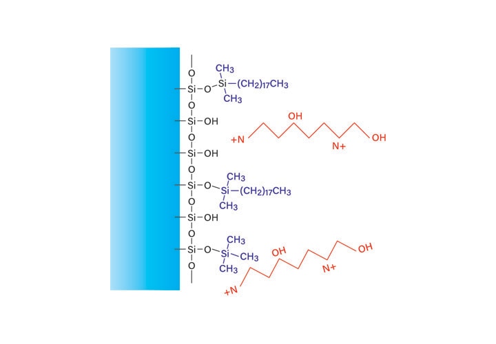
Figure 14: Effect of formic acid on reversed-phase peptide retention.
Formic acid lowers the pH of the mobile-phase, thereby protonating the acidic side chains on the peptide and removing some of the negative charge (Figure 14). The reduced number of charged amino acid side chains increases the attraction to the hydrophobic surface of the column, which promotes better separation. Although most silanols on the surface of the column may also be protonated, free silanols will still be available for binding with the peptide. These peptide-silanol interactions will appear as tailing peaks in the chromatogram.
Trifluoracetic acid (TFA), the most commonly used modifier, differs in the mechanism of interaction with the column and sample (Figure 15). The low pH protonates acidic peptide side chains, and ion pairing neutralizes basic side chains, inhibiting their binding to free silanols which cause peak tailing. The combination of reduced charge and ion-pairing increases the retention, requiring a higher concentration of organic solvent for elution.

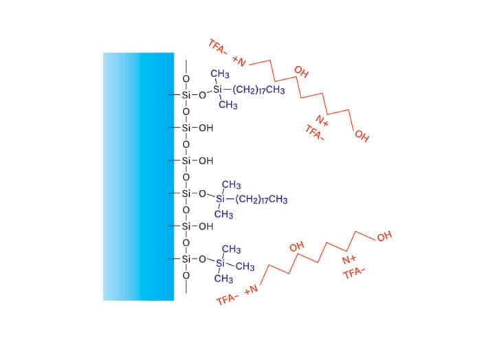
Figure 15: Effect of trifluoroacetic acid on reversed-phase peptide retention.

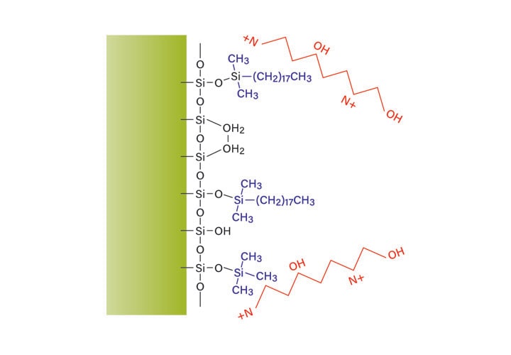
Figure 16: Acidic mobile-phase with hybrid particle column.
The benefit of using a column which has the bridged ethyl hybrid particle is the elimination of silanol interactions (Figure 16). TFA is no longer needed to reduce peak tailing because the base packing has fewer interactions with the peptide. Either formic acid (FA) or TFA can be used, instead, to change the selectivity of the separation while maintaining good peak shape. The difference in retention as well as the change in elution order can be used to adjust purification conditions, as shown in Figure 17. The asterisk identifies the same contaminant peptide in the two separations, confirming the considerable and useful change in selectivity.

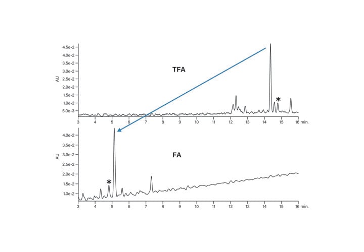
Figure 17: Effect of modifier on the basic peptide.

Role of Elevated pH
Elevating the pH can also be used to change the interaction between the peptide and the bridged ethyl hybrid column surface. With buffers such as ammonium bicarbonate, the high pH deprotonates and ionizes the acidic peptide side chains (Figure 18). The ammonium bicarbonate also deprotonates and neutralizes the basic peptide side chains, which reduces the peptide’s charge and increases its attraction to the hydrophobic column surface. The basic peptide side chains do not bind to the remaining few residual silanols and peak tailing is reduced. In addition to these benefits, ammonium bicarbonate is volatile and relatively easy to remove from the purified peptide product. Ammonium hydroxide, at 0.1%, may also be used to elevate the pH of the mobile-phase and is readily evaporated from collected fractions.

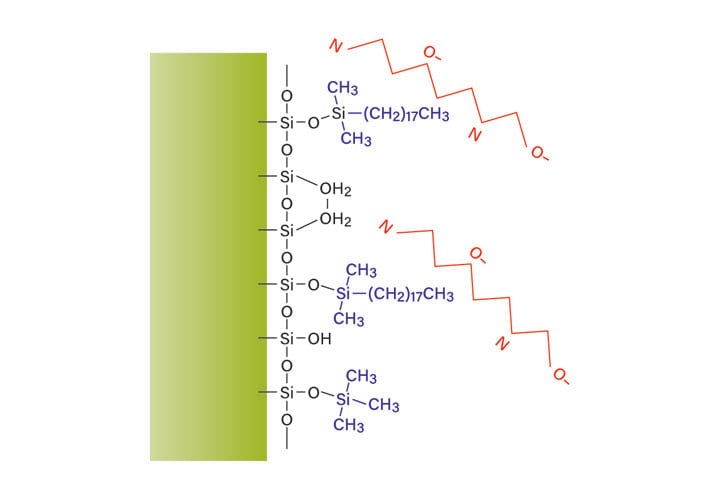
Figure 18: Effect of pH on the reversed-phase retention of peptides.
Extremes of pH change the selectivity of separations (Figures 19 and 20). The acidic peptide (Figure 19) retains better on the reversed-phase packing at low pH because all the negative charges are neutralized and the peptide strongly interacts with the hydrophobic column surface. At high pH, on the other hand, the peptide moves to an earlier retention time due to a greater number of negative charges, which prevent it from adhering as strongly to the column packing. For this example, the peak shape remains unaffected but the change in elution order could be used in method development or to characterize the peptide with an orthogonal strategy. The basic peptide (Figure 20) exhibits the opposite behavior at the extremes of pH, as expected. At high pH, the basic residues of the peptide are deprotonated and non-ionized. The strong interaction of the peptide with the column requires a higher percentage of organic mobile-phase to elute it from the column. The change in selectivity, with improved resolution at pH 10, makes the higher pH more attractive for the end goal of isolating peptide with increased purity.

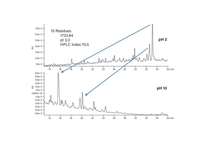
Figure 19: Effect of mobile-phase pH on the acidic peptide (pI 3.3).

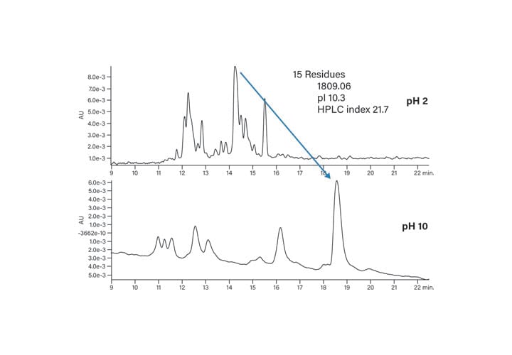
Figure 20: Effect of mobile-phase pH on the basic peptide (pI 10.3).
Reminder: While mobile-phases at both low and high pH are compatible with hybrid particle technology columns, method conditions at the extremes of pH should not be used with silica-based column packings. Excessively low pH will cleave the bonded phase. High pH will destroy the silica particle column substrate. Always check the manufacturer’s suggested pH range limits for specific silica-based columns.

Role of Temperature
Temperature control is most often used in chromatography to ensure reproducible separations. In isolation and purification, it is valuable for several additional reasons. Hydrophobic peptides that have limited solubility are among the most difficult samples to purify. Raising the temperature of the separation increases the solubility of hydrophobic peptides and usually improves their chromatographic peak shape. This ultimately improves the purity and recovery of the isolation, making the isolation faster and more efficient. Since different temperatures give different chromatographic selectivity, column heating is a very convenient tool for optimizing the separation of a particular sample. In addition, mobile-phase viscosity and total system pressure are reduced with elevated temperature. Lower system pressure reduces strain on the system, fittings, and column, and ultimately increases the ruggedness of the operation.
While temperature control in analytical chromatography is routine, temperature is infrequently employed as a parameter for manipulating chromatography at the preparative scale for two reasons. First, large diameter columns cannot be uniformly heated from the outside. Second, high flow rate separations actually occur at the temperature of the incoming solvent. Electric blankets and column ovens, while satisfactory for small scale separations, cannot uniformly heat large columns.20 Temperature gradients form across the diameter and length of the column, adversely affecting the chromatography.
Effective column heating is accomplished by inserting a solvent preheating loop at the head of the column and completely submerging the loop and the column in a water bath equilibrated to the desired temperature (Figure 21). Continuously flowing solvent through the preheating loop brings the column to equilibrium internally, while the water bath stabilizes the external column environment. The amount of band broadening attributed to the solvent preheating loop is negligible because it is constructed with narrow internal diameter tubing. The incoming sample is also re-focused by adsorption to the head of the column.

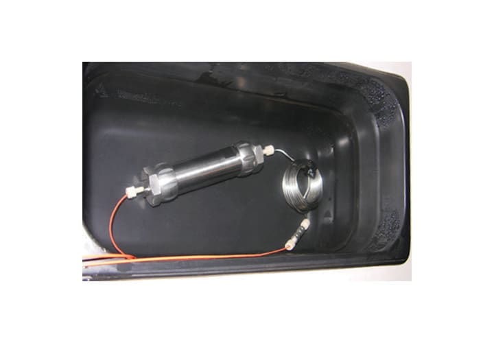
Figure 21: Setup for large column temperature control.
The effect of using temperature control for peptide separations is shown for two of the test panel peptides, the basic peptide (Figure 22) and the acidic peptide (Figure 23). In these examples (highlighted in red), the basic peptide’s sample components are better separated at 60˚C, while the acidic peptide crude mixture components are better resolved at 40˚C. These observations are purely coincidental, however, since predicting the optimal temperature for either acidic or basic peptides is nearly impossible and will depend upon the specific properties of the individual sequences.

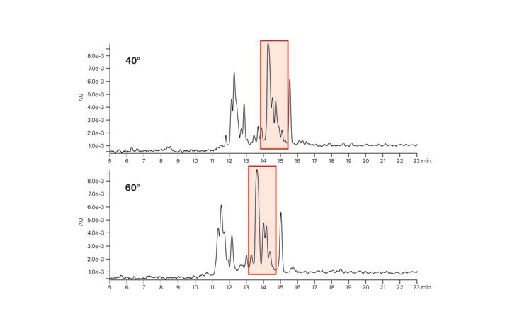
Figure 22: Effect of temperature on the basic peptide.

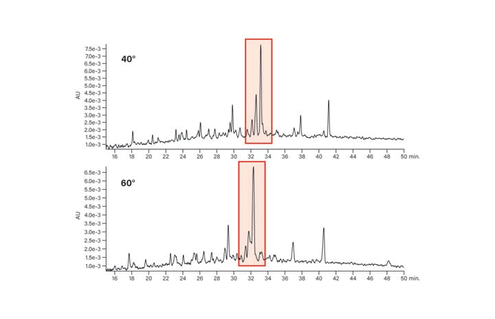
Figure 23: Effect of temperature on the acidic peptide.
Changing the solvent, mobile-phase modifier, pH and temperature dramatically affect peptide separations and any one of these parameters can be used alone or in conjunction with one another as method development tools to optimize chromatography. A single column choice packed with stable hybrid particles, such as the XBridge Peptide BEH Column technology, can simplify the purification process by reducing the number of columns and screening time required for peptide isolation. The chromatography of the basic peptide in Figure 24 illustrates the impact that small changes have on the separation. For those peptides with unique properties, other column chemistries may be useful for optimizing their separation.

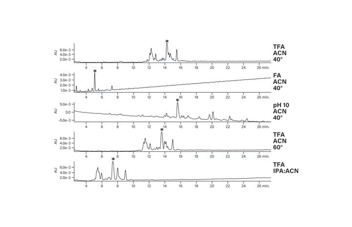
Figure 24: Separation of the basic peptide under various conditions on an XBridge Peptide BEH C18 Column.
Focusing the Gradient
Chromatographic separations for isolation and purification are governed by the same physical and chemical principles as analytical separations. In prep experiments, however, scientists isolate compounds at high mass loads, often on large columns, and require better resolution to enhance purity and recovery of the collected product. Creating a shallow gradient is a good first approach to enhancing resolution, but changing the gradient slope for the whole separation can make peaks broad and increase the total run time. Segmented and focused gradients decrease the gradient slope for only that portion of the separation that requires the increased resolution, without increasing the total run time (Figures 25 and 26).

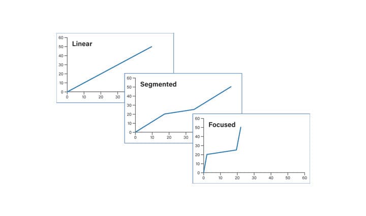
Figure 25: Profiles for linear, segmented and focused gradients.

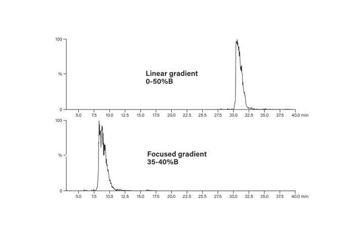
Figure 26: Peptide elution with linear and focused gradients.
Linear gradients progress from low to high organic composition (i.e., 5-50%B or 5-95%B) over the course of a defined time period and are often used for sample screening. They may also be employed for preparative chromatography if there is good resolution between sample components and the run time is reasonably short. Segmented gradients maintain the same slope before and after the shallower, focused portion of the method, preserving the chromatographic profile for these parts of the separation. The shallower, focused portion of the chromatogram has a decreased gradient slope, which effectively moves closely-eluting impurities away from the peak of interest. Focused gradients are intended to target only the product. Solvent strength is rapidly increased from the low concentrations used for sample loading to about 5 percent below the expected elution point for the product peak. In general, the shallow part of the chromatogram proceeds at about one-fifth the slope of the original separation to about 3 percent above the expected elution for the product peak. Once the shallow portion of the gradient is completed, the percentage of organic mobile-phase is quickly increased to wash the column of any remaining contaminants. Because of the complexity of peptide mixtures, often the best resolution is near 0.25%-0.33% change/column volume, a slightly shallower slope than the typical one-fifth of the original screening gradient slope that is employed for small molecules and less complex peptide samples.
The system volume is used in designing the focused gradient,21 as well as in basic scaling from the analytical to preparative scale. The system volume, also called delay volume or dwell volume,22 is defined as the volume from the point of gradient formation to the head of the column and includes all components of the HPLC flow path, pump heads, pulse dampeners, mixers, the injector loop, and tubing. In geometric scaling, where the slope is preserved at both the analytical and preparative scales, the system volume imposes an isocratic hold before the gradient begins. This hold can be several column volumes at the small scale or a fraction of a column volume at the large scale. A programmed isocratic hold at initial conditions is used to compensate for the difference in system volume between the analytical and preparative scales, thus ensuring that the actual gradient starts at exactly the same time.
Using a step gradient (Table 3) where the mobile-phase A solvent is neat and the mobile-phase B solvent contains an appropriate UV absorber (i.e., acetone at 2 mL/L), the system volume can be easily calculated using the procedure and calculations shown in Figures 27 and 28.

Table 3: Step gradients for analytical and preparative system volume determination.

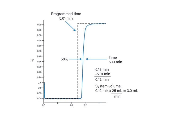
Figure 28: System volume calculation.
While it is possible to estimate the system volume, column volume, and the percentage of strong solvent that elutes the peptide, and then create the segmented or focused gradient from these estimations to save time, it is worthwhile to determine system volume experimentally and record these values for subsequent experiments. The system volume will remain constant as long as there are no modifications to the HPLC plumbing and the method flow rate is identical to the flow rate used to measure the system volume. Once the system volume is determined experimentally, modifications to the system (like changing the size of the injector loop), are easily calculated and do not require additional volume measurement. Once the system volume is determined, it can be utilized in focused gradient calculations.

Designing the Focused Gradient
Focused gradients are usually designed based on the analysis of the crude sample mixture, but the procedure is identical for modifying a gradient which has already been used in an initial preparative run. Using the equations shown below, creating a focused gradient is straightforward. Assume that the following gradient is the one from which the focused gradient will be designed: 4.6 X 100 mm column, system volume 1.0 mL, column volume 1.097 mL*
Peak retention time = 7.76 min

*Column volume may be determined using a calculator available on the web, or by using the volume of a cylinder: V = πr2h. The values will be slightly different depending on the method chosen, because some calculators reduce the liquid volume to account for the column packing. As long as the same method is used for all calculations, there will be no impact on the chromatography.

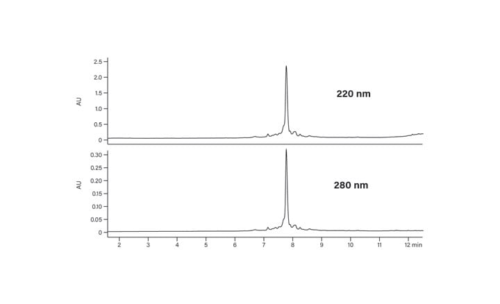
Figure 29: HPLC analysis of the crude synthetic peptide.
Figure 29 shows the chromatogram of the crude synthetic peptide analyzed with this gradient.
Calculate the offset between the point of gradient formation and the detector
Offset = System Volume + Column Volume
Example:
Offset = 1.0 mL + 1.097 mL
Offset = 2.097 mL
Calculate time for the solvent to reach the detector
Time to detector = Offset in mL
Flow rate in mL/min
Example:
Time to detector = 2.097 mL / 1.46 mL/min
Time to detector = 1.43 min

Calculate the time when the peak elution concentration was formed
Time elution concentration =
Peak retention time – Time to detector – Gradient hold
Example:
Time elution concentration = 7.76 min – 1.43 min – 0.00 min
Time elution concentration = 6.33 min

Calculate peak elution %
% Elution concentration =
Time elution concentration / Length Pilot X Change pilot /
Gradient segment + Initial pilot gradient % / Gradient segment
Example:
% Elution concentration = 6.33 min / 10 min X 45% + 5%
% Elution concentration = 33.48%

NOTE: For all calculations involving percent, use absolute values only, i.e., 45 X 6.33 min, not 0.45 X 6.33.

Calculate the pilot gradient slope in % change per column volume
# Column volumes (CV) =
1 CV X Flow rate in mL X Gradient segment time X mL min
Example:
# Column volumes = 1 CV X 1.46 mL X 10 min / 1.097 mL min
# Column volumes = 13.3 CV
Example:
Pilot gradient slope = % change pilot gradient
Pilot gradient slope = 45% / 13.3 CV = 3.38% / CV

Calculate the focused gradient slope in % change per column volume. Use one-fifth of the pilot gradient slope.
Focused gradient slope in %/CV = 1/5 × Pilot gradient slope
Example:
Focused gradient slope = 1 X 3.38% / 5 CV
Focused gradient slope = 0.67% / CV

Create focused gradient segment from 5% below to 3-5% above estimated elution percentage. The peak elutes at 33.5% acetonitrile. The shallow gradient should go from 28% to 36% acetonitrile. Calculate the time for the focused gradient segment.
Time focused gradient segment =
% Change X Focused gradient slope X Column volume X Flow rate in mL
Example:
Time focused gradient segment =
8% X 1 CV / 0.67% X 1.097 mL / 1 CV X 1 min / 1.46 mL
Time focused grad segment = 9.0 min

Write the focused gradient starting at initial conditions of the pilot run and quickly ramping to 5% below the elution % for peak.

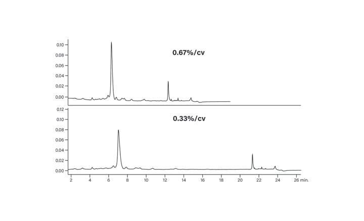
The top panel of Figure 30 shows the chromatogram of the crude peptide analyzed using the focused gradient. The closely eluting impurities are better resolved, but decreasing the slope to about one-tenth the initial slope (bottom panel) gave the best resolution of the impurities. This example clearly illustrates the impact reducing the slope to between 0.25-0.33% change per column volume can have on the separation of a complex peptide mixture. Note that the retention time of the main peptide peak is still about 7 minutes, approximately the same time as for the original screening gradient. Focusing the gradient, therefore, increased the resolution without increasing run time. While overall run time for the total gradient is longer, other techniques such as early run termination can be used to speed up the isolation process at the larger scale. This peptide was ultimately isolated by geometrically scaling the shallower focused gradient.23

Sample Introduction
There is no universal solvent or technique for dissolving synthetic peptides because peptide composition and sequence directly impacts solubility. Useful solvent choices include water with 0.1-2% trifluoroacetic acid, formic acid, or acetic acid, dimethylsulfoxide, hexafluoroisopropanol, 6-12 M guanidine-HCl, dimethylformamide, 0.1% ammonium hydroxide, or 10 mM ammonium bicarbonate. Manufacturers sometimes provide practical guidance for dissolving different types of peptides.24 Dissolving the peptide often results in having a relatively large volume of sample in strong solvent.
In conventional preparative chromatography systems (Figure 31), large injection volumes of strong sample diluents often distort the chromatogram, reducing the amount of product that can be successfully isolated. As the load increases, the resolution of closely eluting impurities is lost. Precipitation of the sample due to the presence of aqueous mobile-phase on either side of the sample in the loop or on the head of the column decreases system ruggedness and column lifetime.

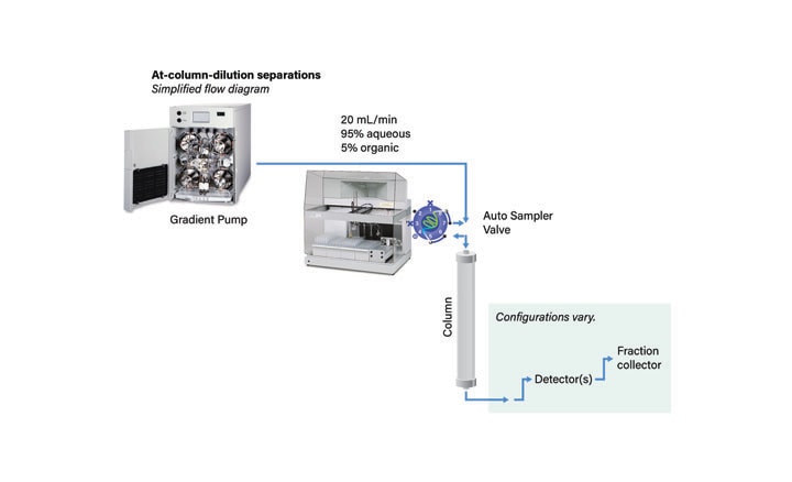
Figure 31: Plumbing diagram for standard gradient system.
In conventional separations, a sample introduced to the column in DMSO, or some other strong solvent, immediately begins to travel down the column, carrying the sample molecules with it (Figure 32). The sample is not retained until the strong solvent is diluted in the column. Unfortunately, by the time the sample bands retain on the column, they are already wide, migrating into one another on the column bed. When the sample components elute from the column, the bands are not distinct and the purity of each component is poor.

Figure 32: Standard preparative separation with DMSO as the sample solvent.
At-Column Dilution25, 26 (ACD), an alternative injection technique, permits the injection of large volumes of strong solvents and concurrently improves sample solubility, column loading, and resolution. With ACD, the chromatographic system is plumbed so that the sample in strong solvent is diluted at the head of the column with aqueous mobile-phase (Figure 33). The sample is very quickly mixed and adsorbed on the column. The rate of transfer is so rapid that precipitation cannot occur. The strong solvent immediately begins flushing from the column before sample elution begins. Once the gradient is initiated, the sample components elute as narrow, low-volume, sharply resolved bands (Figure 34). Improved resolution between sample component peaks permits increasing the sample size and thereby reducing the number of injections required for isolation. In practice, with At-Column Dilution, the column loading can often be increased by three to five fold (Figure 42). System ruggedness is improved with At-Column Dilution since the sample has limited ability to precipitate in the loop or at the column head.
The incidence of high-pressure shutdowns is reduced and column lifetime is extended.

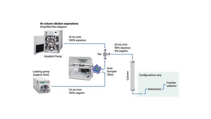
Figure 33: Plumbing diagram for system with At-Column Dilution.

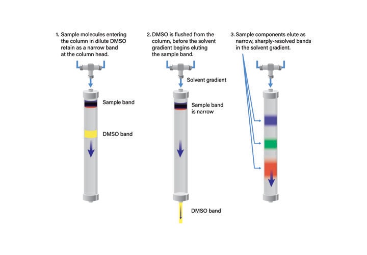
Figure 34: At-Column Dilution preparative separation with DMSO as the sample solvent.

PRACTICAL PEPTIDE ISOLATION EXAMPLE
The principles of prep chromatography apply to all types of molecules, including peptides. The following example illustrates a typical workflow for isolating a peptide in a research environment and applies the factors for method optimization presented above. The procedure may be modified depending upon the process requirements of the laboratory.
The peptide used in this example was 17 amino acids in length with 3 basic, 2 acidic, 8 nonpolar, and 4 polar residues. The sample was dissolved in dimethylsulfoxide, with vortexing and sonication, and then passed through a 0.45 µm GHP Acrodisc syringe filter. The peptide monoisotopic mass was 1772.9 Da and had the following charge states:
[M+H]+ = 1773.9
[M+2H]2+ = 887.5
[M+3H]3+ = 592.2
[M+4H]4+ = 447.2

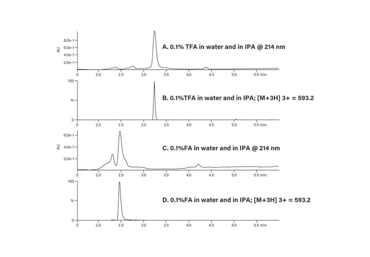
Figure 35: Crude peptide analysis with TFA and FA modifiers.

Crude Peptide Profile
The crude peptide sample was analyzed with two different modifiers (0.1% formic acid and 0.1% trifluoroacetic acid) in the mobile-phase to determine which would give the better separation. While acetonitrile is most often used as the organic component of the mobile-phase, in this example, isopropanol was used instead for purposes of illustration. The results are shown in Figure 35, where the TFA modifier (A and B) produced a sharper product peak with well-resolved contaminants when compared to formic acid (C and D), all at 40˚C. The separation was also evaluated at 25˚C and 60˚C, but 40˚C showed the best peak shape and resolution of the sample component peaks (Figure 36). The slightly elevated temperature also reduced the system backpressure attributed to isopropanol as the organic component of the mobile-phase.

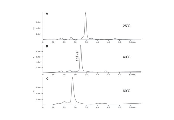
Figure 36: Evaluation of the crude peptide separation at three temperatures.

Focusing the Gradient
After the mobile-phase modifier and temperature were optimized for the analysis of the crude, focusing the gradient was used to improve the resolution of closely-eluting contaminant peaks. The 4.6 × 50 mm column had a volume of 0.698 mL and the system volume was measured at 0.77 mL. The HPLC method used for the crude peptide analysis is shown below:

Calculate the offset between the point of gradient formation and the detector
Offset = System volume + Column volume
Example:
Offset = 0.77 mL + 0.698 mL
Offset = 1.468 mL

Calculate time for the solvent to reach the detector
Time to detector =
Offset in mL / Flow rate in mL/min
Example:
Time to detector = 1.468 mL / 1.46 mL/min
Time to detector = 1.00 min

Calculate the time when the peak elution concentration was formed
Time elution concentration =
Peak retention time – Time to detector – Gradient hold
Example:
Time elution concentration = 3.23 min – 1.00 min – 0.50 min
Time elution concentration = 1.73 min

Calculate peak elution %
% Elution concentration =
Time elution concentration / Length pilot X Change pilot / Gradient segment +
Initial pilot gradient % / Gradient segment

Example:
% Elution concentration = 1.73 min X 30% + 0% / 4.78 min
% Elution concentration = 10.85%

NOTE: For all calculations involving percent, use absolute values only, i.e., 30 × 1.73 min, not 0.30 × 1.73.

Calculate the pilot gradient slope in % change per column volume
# Column volumes (CV) =
1 CV X Flow rate in mL X Gradient segment time X mL min
Example:
# Column volumes = 1 CV X 1.46 mL X 4.78 min / 0.698 mL min
# Column volumes = 9.99
Pilot gradient slope = % Change pilot gradient
# column volumes
Example:
Pilot gradient slope = 30% / 9.99 CV = 3.0% / CV

Calculate the focused gradient slope in % change per column volume. Use one-fifth of the pilot gradient slope.
Focused gradient slope in %/CV =
1/5 X Pilot gradient slope
Example:
Focused gradient slope = 1 X 3.0% / 5 CV
Focused gradient slope = 0.6% / CV
Create focused gradient segment from 5% below to 3-5% above estimated elution percentage. The peak eluted at 10.85% acetonitrile, therefore, the shallow gradient was designed to run from 5-13% acetonitrile in 6.37 min.
Time focused grad segment =
% Change X Focused gradient slope X Column volume X Flow rate in mL
Example:
Time focused grad segment = 8% / 0.6% X 0.698 mL / 1 CV X 1 min / 1.46 mL
Time focused grad segment = 6.37 min
Write the focused gradient starting at initial conditions of pilot run and quickly ramp to 5% below the elution % for peak.

Once the focused gradient was created, the crude peptide sample separation was evaluated (Figure 37A). A small impurity peak eluted just prior to the product peak, but it was barely perceptible. At double the load (Figure 37B, 72 µg), the impurity was more visible, but the main peak was still relatively pure. Four times the original load of 36 µg produced a chromatogram where the impurity was more pronounced and would most likely reduce the probability of obtaining pure product if this load was geometrically scaled to the larger column for prep (Figure 37C). With a
256 µg load on the analytical column, the impurity completely coeluted with the main peak (Figure 37D).

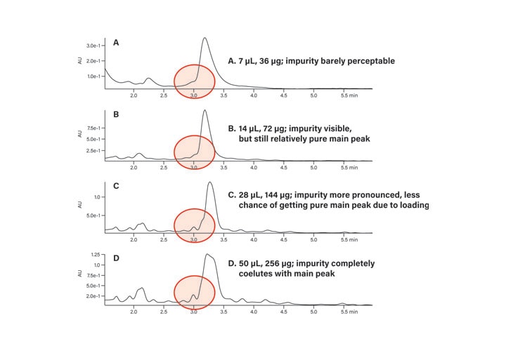
Figure 37: Loading study using the focused gradient on the analytical column.

Scaling to Prep
The 72 µg load on the analytical column was selected for geometric scaling to prep. This conservative load would increase the probability of obtaining a reasonable amount of pure material with fewer injections than scaling the lowest injection volume.
Mass load is proportional to column volume and is determined using a prep calculator or by solving for M2 in the following equation where:
M1 is the mass loading on column 1 M2 is the mass loading on column 2
L1 is the length and d1 is the diameter of column 1 L2 is the length and d2 is the diameter of column 2
M2 = M1 X L2 / L1 X d22 / d12
M2 = 72 μg X 100 mm / 50 mm X 19 mm2 / 4.6 mm2
M2 = 72 μg X 36,100 / 1058
M2 = 2456 μg or 2.4 mg
44.03 mg of crude peptide was dissolved in 5 mL DMSO and filtered (concentration 8.80 mg/mL). Geometric scaling of the 72 µg load on the 4.6 × 50 mm analytical column to the 19 × 100 preparative column required a 2.4 mg injection, as calculated above. With a crude peptide concentration of 8.80 mg/mL, the injection volume was calculated:
Injection volume = 2.4 mg X 1 mL / 8.80 mg/mL
Injection volume = 0.272 mL or 272 μL
The analytical focused gradient was scaled to prep, taking into account the system volumes at both scales (Table 4). While the dwell volume appeared to be high for the preparative system, it included a 5 mL preheating loop for column heating, as well as a 2 mL injection loop. Considering these contributions to the system volume, the 2.75 mL attributable to the remaining system tubing was quite reasonable. The product peak was collected by time (Figure 38).

Column: 4.6 × 50 mm Column: 19 × 100 mm
System dwell volume: 0.77 mL System dwell volume: 9.75 mL
Column volume: 0.698 mL Column volume: 23.804 mL
System dwell volume (in column volumes): 1.10 System dwell volume (in column volumes): 0.41 Gradient offset: 0.66

Table 4: Gradient scaling.

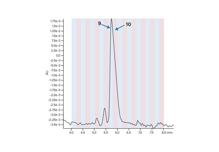
Fraction Analysis
The peptide product peak was collected in two fractions. These two fractions were very pure, as shown in Figure 39. The broad peak which eluted at about 2.25 minutes in each of the fraction analyses and in the blank was most likely from the low concentration of the ion-pairing trifluoroacetic acid modifier in the mobile-phase.27 The hydrophobic constituents in the TFA commonly build up on the column and then elute during the gradient. The contaminant did not come from any system components, such as the injector or valving, as another blank without the column showed no peaks in the chromatogram (Figure 40).

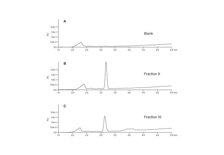
Figure 39: Fraction analysis.

At-Column Dilution
Even though the peptide was isolated with high purity, increasing the sample load per injection would improve process efficiency and reduce the number of chromatographic runs required to purify the requisite amount of product for ensuing experiments. As discussed earlier, At-Column Dilution very effectively manages higher sample loads with a simple system plumbing change (Figure 33).
Although the rate of change of %B per column volume for the peptide isolation using At-Column Dilution was the same as the method used for the conventional, geometrically-scaled separation, the programmed gradient table was modified to include the contribution of the organic solvent introduced by the auxiliary sample loading pump (Table 5).

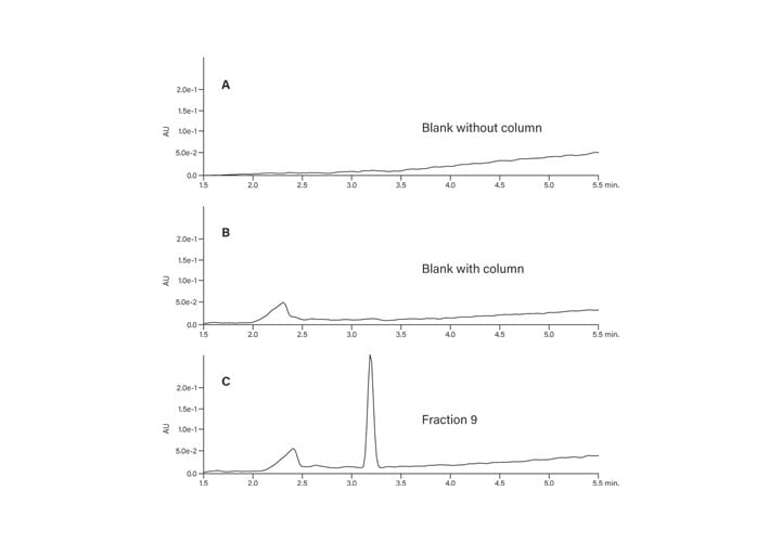
Figure 40: Hydrophobic constituents in TFA.

Gradient time: 14.40 - 1.66 = 12.74 min Gradient time: 16.00 – 3.26 = 12.74 min
Gradient volume: 12.74 min × 25 mL/min = 318.5 mL Gradient volume: 12.74 min × 25 mL/min = 318.5 mL
Column volumes: 318.5 mL × 1 CV/23.804 mL = 13.38 CV Column volumes: 318.5 mL × 1 CV/23.804 mL = 13.38 CV
Gradient slope: 8%/13.38 CV = 0.6%/CV Gradient slope: 8%/13.38 CV = 0.6%/CV
Loading pump flow rate during gradient = 1.25 mL/min
1.25 mL/min = 5% of the total flow
Total gradient method flow rate = 25 mL/min

Table 5: Gradient comparison: conventional and At-Column Dilution methods.
The At-Column Dilution pump introduces organic solvent directly to the sample loop and is programmed to run at 5% of the total flow rate. The flow rate on the chromatographic pump is, therefore, decreased from 25 mL/min in the conventional method to 23.75 mL/min in the At-Column Dilution method. Note that the total flow rate is still 25 mL/min (23.75 mL/min + 1.25 mL/min). Because the At-Column Dilution pump is plumbed directly to the injector, a hold step at initial condition, long enough to ensure complete transfer of the sample from the loop to the column, is inserted at the beginning of the gradient. This system is configured with a 2 mL loop and the original hold step was 0.66 min. Calculating the hold step for the At-Column Dilution method: 2 mL loop x (1 min/1.25 mL)=1.6 min
1.60 min + 0.66 min hold step from the original prep method = 2.26 min hold step for the At-Column Dilution method.
The gradient method percentages of A and B are also modified to reflect the contribution of the At-Column Dilution pump. The focused gradient starts at 5%B and proceeds to 13%. Because 5% of the total flow is delivered at a constant flow rate of 1.25 mL/min isopropanol by the At-Column Dilution pump, the percentages of B in the At-Column Dilution method are programmed as 0% and 8%B, respectively. Note that while the At-Column Dilution method is programmed slightly differently, the actual gradient is identical to the conventional method. Because this peptide elutes at such a low percentage of B, the actual time spent at 5% B is longer in the At-Column Dilution method, incorporating the time spent changing from 0%B to 5%B in the conventional prep method into the hold time in the At-Column Dilution method. These two steps are programmed on separate lines in the At-Column Dilution method for purposes of clarity to the reader. Since the percentages of B are decreased to account for the 5%B delivered by the At-Column Dilution pump, the percentages of A must be increased by 5% to keep the gradient identical to the original conventional injection method. If the chromatographic system has washing steps in the injection sequence, ensure that all wash lines are primed and filled with strong wash solvent.
Because the geometrically-scaled large scale isolation was performed at 40˚C, the temperature was maintained for the injection using At-Column Dilution. The solvent preheating loop was inserted just before the tee in the aqueous solvent stream (Figure 41).

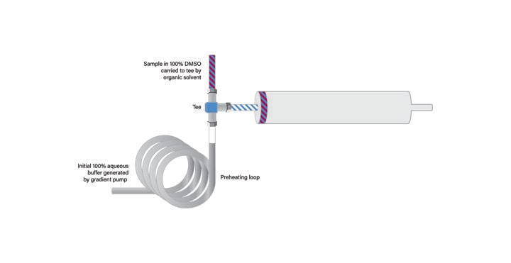
Figure 41: Sample loading with At-Column Dilution and temperature control.
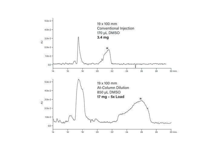
The solvent preheating loop, tee, and column were then submerged in the water bath. Prior to starting the gradient separation, the pressure was allowed to stabilize, which implied system equilibration had been reached. While 2.4 mg of peptide was the maximum amount of sample that could be injected using the conventional plumbing configuration, five times that amount, or 12 mg (1.36 mL), was introduced to the column with the system in the At-Column Dilution configuration (Figures 42 and 43). The fractions were collected by time and subsequently analyzed using the original 0-30%B screening method. The fractions showed excellent purity and were comparable with the fractions collected from the prep which used the conventional injection technique (Figure 44).

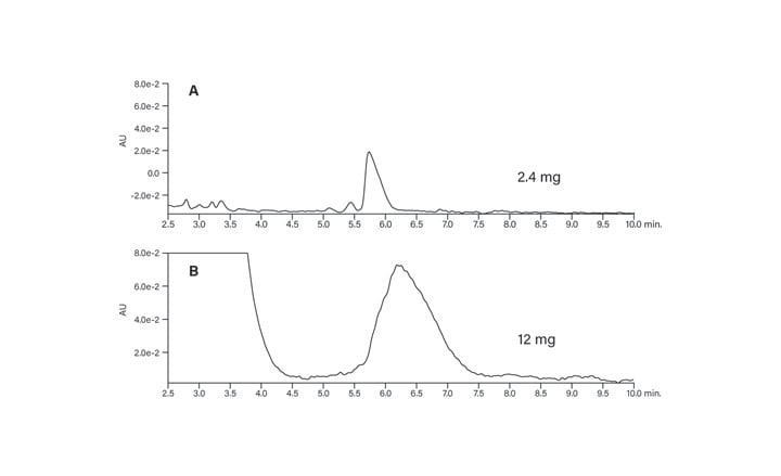
Figure 42: Comparison of conventional and At-Column Dilution sample loading.

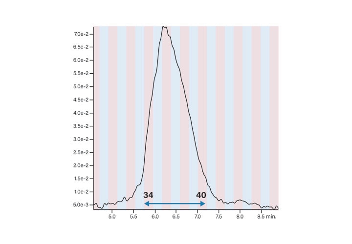
Figure 43: Prep with At-Column Dilution.

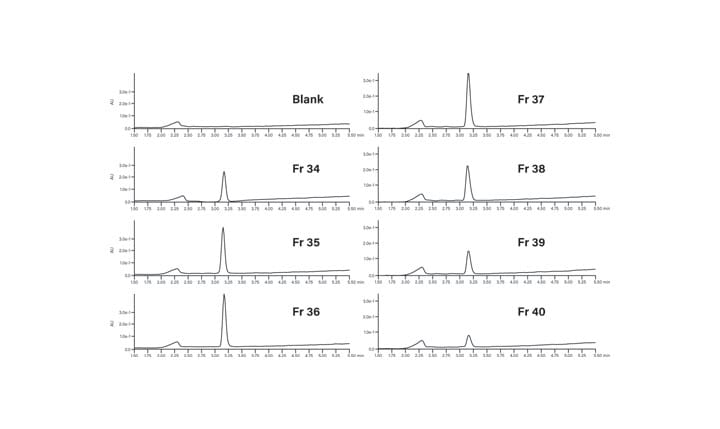
Figure 44: Fraction analysis from the isolation using At-Column Dilution.

Special Considerations for Hydrophobic Peptides
A hydrophobic peptide composed of 12 nonpolar and 3 polar, uncharged amino acid residues was dissolved in dimethylsulfoxide. The preparative focused gradient below was used for isolation on a 19 × 100 mm column with the chromatographic system plumbed for conventional injection. The extreme hydrophobicity of the peptide required using a reduced flow rate,28 lower sample loading, and a temperature of 60˚C.

Although this peptide is a good candidate for using At-Column Dilution, increasing the mass load on the column poses the risk of precipitation. Since the peptide elutes at about 50% acetonitrile, loading this sample at 5% B (as in the previous example) is so far below the required elution strength that the peptide is prone to precipitation as it is diluted at the head of the column. Increasing the percentage of organic solvent coming from the chromatographic pump during the loading step alleviates the potential precipitation problem. Generally, for extremely hydrophobic compounds, using an initial percentage of organic solvent in the gradient method that is 20-25% below the expected compound elution percentage prevents sample precipitation, while preserving the benefits of the At-Column Dilution technique. The modified At-Column Dilution gradient below was used to load a five-fold larger sample on the 19 × 100 mm column (Figure 45).

The gradient started at 48%B (43.6%B + 5%B from the At-Column Dilution pump) and ended at 53% acetonitrile in 29 minutes with a slope of 0.49% change per column volume, identical to the rate of gradient change used for the conventional injection. The At-Column Dilution pump carried the peptide sample from the 5 mL loop to the tee in 100% acetonitrile, where it met the chromatographic pump mobile-phase at its initial condition, 23.6% B (18.6%B + 5%B from the At-Column Dilution pump). The 9.2 minute hold at the beginning of the method ensured the sample was completely loaded onto the column. The At-Column Dilution pump ran at a constant flow rate of 0.8 mL/min, which was 5% of the
16.3 mL/min total flow rate.

Cleaning the Column
All columns require cleaning occasionally, whether they are used for small or large molecule separations. High backpressure, high chromatographic background and extraneous peaks that cannot be attributed to sample are all indications that the column needs cleaning.
Preventing the buildup of contaminants on the column is the best way to extend the life of the column. Filtering all samples before injection is recommended. Adding an in-line filter or guard column prior to the column helps to trap particulates and other undesirable mixture components. Washing the column with two to three column volumes of a high percentage of organic solvent after each separation is useful for systematically removing unwanted contaminants. Finally, At-Column Dilution keeps samples in solution, preventing high pressure shutdown, and effectively passing sample components through the purification system whether their final destination is a fraction collection tube or the waste can.
High backpressure that occurs suddenly is most likely due to sample precipitation somewhere in the system – in the sample loop, the tubing, the column or the detector flow cell. With the chromatographic system pumping, methodically loosening the HPLC fittings starting from the waste line and working back toward the pumps will definitively isolate the source of the high pressure. A gradual increase in backpressure is probably a result of impurity buildup on the column after several injections and may be rectified in a number of different ways. Running repetitive fast gradients at elevated temperature, washing the column for an extended time in a high percentage of organic solvent, or injecting a “cleaning solvent” such as DMSO or 1-10% formic acid may all be used to remove undesirable contaminants on the column (Figure 46).

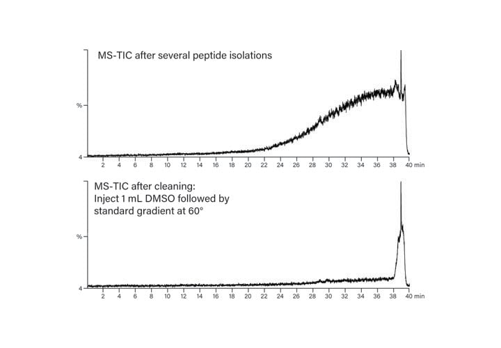
Figure 46: Column cleaning.
Depyrogenation, the removal of endotoxic polysaccharides29 from the column which could contaminate the final product and induce an allergic reaction, commonly requires strong washing with 1 M sodium hydroxide for one hour or more. This procedure is incompatible with current columns.