PRINCIPLES OF SCALING IN PREP SFC
ANALYTICAL METHOD CONSIDERATIONS
When an analytical method is going to be scaled-up for purification purposes, it is important that the chromatography is the best possible for the application. Better resolution at the analytical scale means better chromatography at the prep scale, resulting in higher throughput and purer fractions. The analytical methods also have to take into account the conditions of the preparative technique like column heating, injection mode, pressure drops, system pressure, and matching columns. If purification is by MS, then all screening and method development at the analytical scale should also be done using MS detection. For gradient methods, the slope of the gradient and the equilibration time need to account for the difference in volumes between the analytical and preparative systems. The diluent effect needs to be taken into account as well, since many times the analytical loading is done using mixed-stream injections, while the preparative method uses modifier-stream injections.
LOADING
Keeping in mind the difference in injection strategies (discussed in Chapter 3), loading studies are typically done on the smaller (analytical) scale first. It is important to know about the solubility of the compounds in a sample before introducing it to the system. The best practice in preparative applications is to be able to load the most sample in the least amount of solvent (highly concentrated samples). However, the sample also has to stay in solution after being introduced to the combined CO2 and organic mobile phase. Once an acceptable concentration has been determined, a sample loading
study is conducted where the injection volume is incrementally increased until resolution is lost, or the chromatography is no longer usable for obtaining pure fractions of the target compounds.
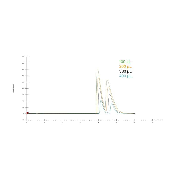
Figure 31 shows an example of a loading study using an optimized isocratic method. Resolution is lost at injection volumes higher than 200 µL in this example, so 200 µL injections would be used either for purification, or in calculating the loading for a scaled-up separation.
GENERAL REQUIREMENTS OF SUCCESSFUL SCALING
Once an acceptable method has been developed and a loading study has been completed at the analytical scale, it is ideal for the retention and selectivity to be the same (or similar) on scale-up.⁹ To successfully scale the chromatography, several parameters need to remain constant:
■ The mobile phases need to be identical; in SFC this means an identical co-solvent (solvent B), and that the CO2 needs to be of similar quality, inlet pressure, physical state (liquid or gas) and delivery method.
■ The columns need to be the same chemistry, length, and particle size to provide the best chance at matching chromatography at different scales. If small particle size columns are being used at the analytical scale, then the ratio of length to particle size (L/dp) must be the same between columns.
■ The samples need to be the same concentration, and dissolved the same diluent.
GEOMETRIC SCALING
In Prep SFC, just like in LC, the injection volumes (loading) and flow rates are scaled geometrically.
To maintain peak shape and loading capacity the injection volume needs to be scaled appropriately for the column size. The capacity is determined by the following equation:
where Vol is the injection volume (µL), D is the inner diameter of the column (mm), and L is the column length (mm) [20].
Similarly, to maintain separation quality, the flow rate is scaled based on the column dimensions. With columns of an identical length and particle size, the geometric scaling of the flow rate is as follows:
where F is flow rate (mL/min) and D is the inner diameter of the column (mm).20
DWELL VOLUME AND EXTRA-COLUMN VOLUME
When columns are of identical length, changes to the gradient profile in the preparative method are required based on the dwell volume. To make these adjustments, the dwell volume must be measured for both the analytical and preparative system. To determine dwell volume, usually a compound or solvent that provides UV signal is added to the co-solvent and a gradient is run without a column. Based on the time delay between the gradient start at the pumps, and the change in signal at the detector, the dwell volume can be determined by multiplying the time delay by the flow rate (Figure 32).
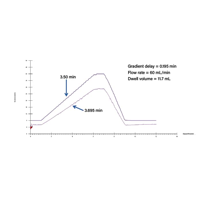
Figure 32. Data generated to determine system dwell volume using 1% acetone in methanol as the co-solvent. Gradient conditions were as follows: hold at 5% for 1 minute, 5 to 40% in 5 minutes, hold at 40% for 1 minute, 40 to 5% in 2 minutes, and hold at 5% for 1 minute. The column was removed from the system to generate this data.
It is also important to note the impact of any extra-column volume such as tubing, injection valves, loop size, detector flow cells and splitters that can result in band broadening in the final chromatography.⁶ To measure extra-column volume and band broadening, the column is removed and an injection is made. The time between the injection and detection, multiplied by the flow rate equals the extra-column volume. The peak shape without a column indicates any broadening occurring as a result of the extra-column volume. Figure 33 shows an example injection done to measure extra- column volume. Because the system was plumbed for modifier-stream injection, the injection was made with 100% co-solvent, so the volume could be determined more accurately and without the addition of CO2 post injection. Details on this procedure are included in the Preparative OBD Column Calculator, an online application which can be accessed at www.waters.com. The column calculator provides an easy to use tool that aids in all of the analytical-to-preparative scaling calculations.
MOBILE PHASE DENSITY CONSIDERATIONS
The simple scale up rules for LC, while applicable in SFC, cannot be applied directly since they assume constant density of the mobile phase. Scale-up in SFC is more complex, mainly due to the compressibility of the mobile-phase causing density, pressure and temperature variations across the column and between systems. Variations in these factors have an impact on mobile phase composition and strength.⁹ The resulting effects on retention and selectivity make it more difficult to maintain the separation profile between analytical and preparative scale systems.
The density and temperature variations cannot be directly controlled, but the chromatography can be successfully matched across multiple scales by adjusting the following method parameters in SFC:
■ Matching the average pressure (and thus the average density) between systems. The average pressure equals the sum of the front and back pressures divided by two. The pressures can be matched by changing the automated pressure regulator setting on either the analytical or the preparative instruments to maintain similar pressure (density) profiles across the column. It should be noted that matching average pressure will not always ensure a matched density profile, however the profiles will show better agreement.
■ Precise matching of the mobile phase composition of carbon dioxide and co-solvent. This is basically a unit conversion between systems from volume-flow to mass-flow (on the analytical) or mass-flow to volume-flow (on the prep) to have equivalent mobile phases.
In SFC, co-solvent composition is the most important parameter that controls peak retention. As a result, accurately scaling of the co-solvent composition is essential for scale-up of the method. By matching the mass flow and composition of the CO2 and co-solvent together with column outlet pressure and temperature, reliable scale-up is possible from a volume-flow based instrument to a mass-flow based instrument.⁹
EXAMPLE SCALE-UP
In this example, the analytical method was developed on the UPC2 system with the following parameters (table 8):
|
Analytical method parameters
|
|
Flow rate
|
3 mL/min
|
|
Co-solvent
|
Methanol
|
|
Composition
|
89:11 CO2
|
|
Back pressure
|
120 bar
|
|
Temperature
|
35 ºC
|
|
Injection volume
|
10 µL
|
|
Column
|
4.6 x 150mm, 5 µm, Chiralpak IA
|
Table 8. Optimized UPC2 analytical method parameters used to scale-up to a preparative SFC system.
In order to maintain constant column length and particle size, a 21x150mm Chiralpak IA column with 5 µm particles was used on the preparative system. The injection volume was scaled geometrically, so the 10 µL injection on the 4.6 mm I.D. column equated to a 208 µL injection on the 21 mm I.D. column. In this case, the CO2 pump on the analytical system was volume-flow controlled, while the pump on the preparative system was mass-flow controlled. As a result, the analytical method CO2 flow rate had to be converted to mass-flow before calculating geometric scale-up. This was done using the following equation.
■ CO2 flow = 2.67 mL/min
■ CO2 density = 0.89 g/mL
■ CO2 flow (mass) = CO2 flow x CO2 density
■ CO2 flow (mass) = 0.89 x 2.67 = 2.38 g/min
Since the co-solvent scales normally (mL to mL) and the co-solvent flow rate was 0.33 mL/min, the total analytical flow rate was 2.70 g/min at approximately 12% methanol. This flow rate and percentage were scaled geometrically, resulting in a preparative flow rate of 56 g/min on the 21 x 150mm column at 12% co-solvent conditions.
Once the flow and composition were determined, the density profile had to be matched to the analytical system using the same average pressure. The front pressure on the analytical system was 162 bar and the back pressure was 120 bar (pressure drop was 42 bar), so the average pressure was calculated to be 141 bar. Since the pressure drop on the preparative system was only 24 bar the back pressure had to be set to 130 bar in order to match the average pressure from the analytical system. Finally, the temperature was also matched at 35 °C. Using these parameters, successful scale-up of the separation from the ACQUITY UPC2 to the Prep SFC system is shown in Figure 34. The profiles are the same, however there is a slight increase in retention on the prep system, likely due to the difference in injection strategy. The analytical system used mixed-stream injection, while the prep system used modifier-stream injection.
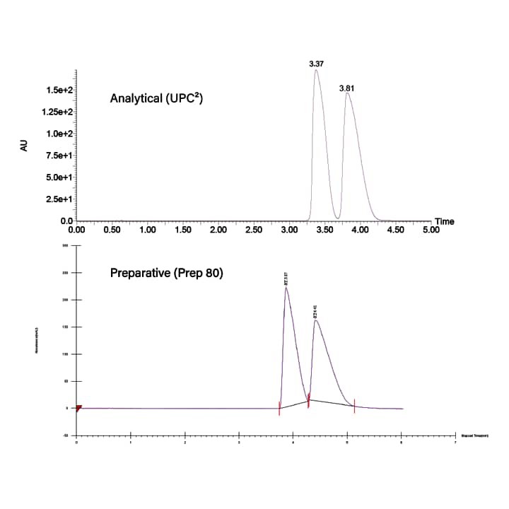
Figure 34. Example scale-up of a chiral separation from the UPC2 system to a Prep SFC system.
STACKING INJECTIONS
For many applications, stacked injections are used. Stacked injections reduce the time between injection cycles and minimize solvent usage. Stacked injections also significantly improve throughput by utilizing all of the available chromatographic space for continuous separation and purification. Usually, injections are made while an already injected sample is on (or eluting from) the column. Therefore, to utilize stacked injections, isocratic methods are required. In order to stack injections successfully, the correct cycle time (or time between injections) needs to be determined. Also, the total run time is required for the last injection in the sequence to ensure all sets of peaks are eluted and collected. Figure 35 shows how these values are determined, and then applied in a set of stacked injections. Because the cycle time is around half of the total run time, two injections are made before the first target peak even begins eluting. After the last injection is made, two sets of peaks elute and are collected. In this case, using stacked injections cuts the total processing time in half when compared to conventional single injection runs.
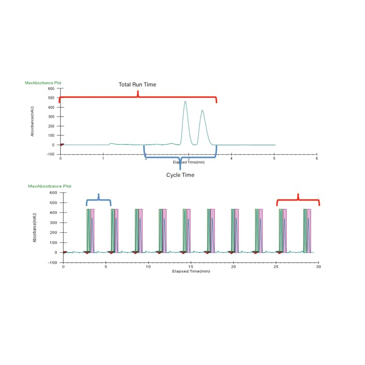
Figure 35. Chromatograms showing how cycle time is determined based on a scouting run (A) and then applied to a set of stacked injections (B). The cycle time is indicated in blue, and is less than 2 minutes. The total run time is indicated in red, and is approximately 4 minutes.
EXAMPLE APPLICATIONS
Due to the expanded selectivity range of SFC described previously, the technique is suited to a wide variety of applications (Table 9).
|
Market area
|
Applications
|
|
Natural Products
|
Traditional medicines Essential oils
Flavors and fragrances Tobacco
Fish oil Cannabis
Chemical markers/product confirmation
|
|
Pharmaceutical
|
Chiral purification
Pharmaceutical discovery compound isolation Impurity profiling/isolation
Steroids
Beta-blockers/nsaids Cannabinoids
Anti-depressants
|
|
Chemical Materials
|
OLED
Polymers
PET agents (positron emitting isotopes) Petrochemical
|
|
Food & Envronmental
|
Lipids/fatty acids Vitamins Steroids
Flavors Pesticides
Carotenoids and antioxidants
|
|
Forensics
|
Illicit drugs – Opiates, steroids, catinones Cannabis
Chemical markers Adulterants
|
Table 9: Preparative SFC applications by market area.
Regardless of the market area or goal of the purification, Prep SFC provides:
■ Diverse selectivity in a single, easy to use, platform
■ Range of chromatographic scaling
■ Increased productivity and solvent savings
■ Orthogonality to reversed-phase LC
■ Separation and purification of compounds with structural similarity
In this section, excerpts from example applications are presented to showcase different workflows and application areas. All of these applications are viewable in their entirety on the Waters website www.waters.com.
CHIRAL PURIFICATION OF VOLATILE FLAVORS AND FRAGRANCES BY SFC
https://www.waters.com/webassets/cms/library/docs/720005150en.pdf²¹
One of the key application areas of SFC is chiral separations. Just as the enantiomers of chiral drugs exhibit different pharmacological activity, the stereochemistry of flavor and fragrance compounds dictates taste, odor quality, and intensity. Purification of these compounds can be quite challenging due to their volatility. SFC offers a fast, low temperature, option for high recovery of chiral flavor and fragrance compounds.
Here, the enantiomers of linalool and terpinen-4-ol were purified from lavender and tea tree essential oils, respectively, using chiral Prep SFC with stacked injections. Figure 36 shows scale-up of the analytical methods on the 4.6 x 250 mm AD-H column to the semi-prep 10 x 250 mm AD-H column. The tea tree oil separation shows both terpinen-4-ol enantiomers are present, while the lavender oil contains only one of the linalool enantiomers. The Prep SFC method parameters are displayed in Table 10.
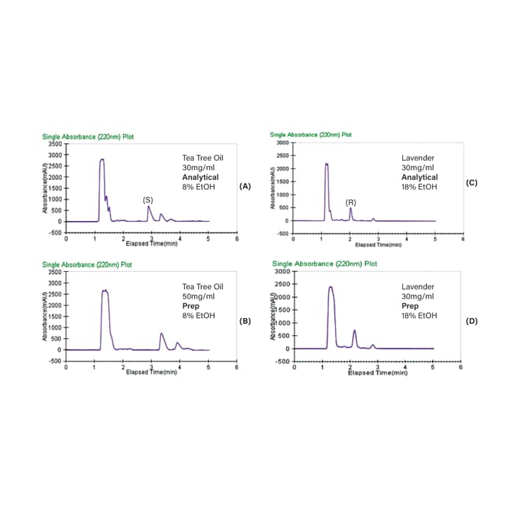
Figure 36. Optimized analytical and preparative separations of tea tree oil (A and B) and lavender (C and D) at isocratic conditions.
|
Preparative SFC Conditions
|
|
|
|
Column
|
Chiralpak AD-H, 5 µm, 10 x 250 mm
|
|
|
Mobile phase A
|
CO2
|
|
|
Mobile phase B
|
|
|
|
Collection make-up solvent
|
|
|
|
Total Flow Rate
|
12 mL/min
|
|
|
|
Tea Tree Oil
|
Lavender Oil
|
|
%B (isocratic)
|
8
|
18
|
|
BPR pressure
|
120 Bar
|
120 Bar
|
|
Oven temperature
|
30°C
|
35°C
|
|
Collection make-up flow
|
2 mL/min
|
1.5 mL/min
|
|
Collection temperature
|
35°C
|
25°C
|
|
Sample concentration
|
50 mg/mL
|
30 mg/mL
|
|
Injection volume
|
100 µL
|
100 µL
|
Table 10. Preparative SFC method conditions used to purify terpenin-4-ol and linalool from tea tree oil and lavender oil respectively.
The methods were isocratic, so stacked injections were used, maximizing collection efficiency. Based on the chromatography, the cycle time was approximately 3 minutes for the tea tree oil, and 2 minutes for the lavender oil. The resulting chiral purification using stacked injections is displayed in Figure 37, where 50 mg of the tea tree oil was processed in under 40 minutes, and 30 mg of lavender oil was processed in under 30 minutes.
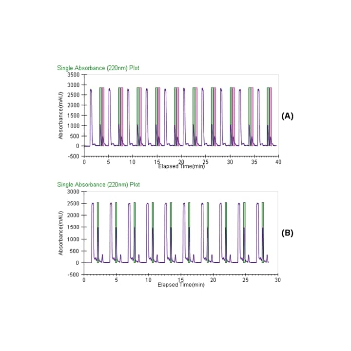
Figure 37. Chromatograms showing stacked injections and collections for (A) tea tree oil and (B) lavender oil.
Fraction analysis is displayed in Figure 38 where the purity for all three fractions was greater than 92%. Recovery studies were performed using racemic standards of the terpinen-4-ol and linalool resulting in 70–80% recovery, which was notable given the fairly low recoveries typically reported.
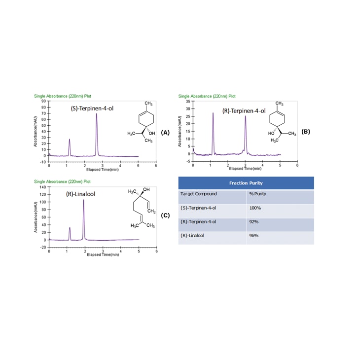
Figure 38. Fraction analysis of the tea tree oil and lavender oil fractions.
ACHIRAL PURIFICATION OF A PHARMACEUTICAL COMPOUND USING MS BASED FRACTION TRIGGERING
https://www.waters.com/webassets/cms/library/docs/720005064en.pdf22
With UV directed purification, the peaks cannot be distinguished from one another by the detectors. Many compounds absorb at the same wavelength. Mass-directed purification collects fractions based on mass, which is a much more specific parameter because it distinguishes between the target(s) and any impurities. When active pharmaceutical ingredients are synthesized, there are sometimes intermediate impurities present with the final product.
Imatinib is a tyrosine-kinase inhibitor used in the treatment of multiple cancers. Here, the reaction intermediate and final products were purified for the synthesis of Imatinib. In the first step, the mixture was screened using three achiral columns and methanol with and without an ammonium hydroxide additive. The results of the screen are shown in Figure 39. The BEH 2-EP column and methanol with ammonium hydroxide were chosen as the best method parameters for optimization and scale-up.
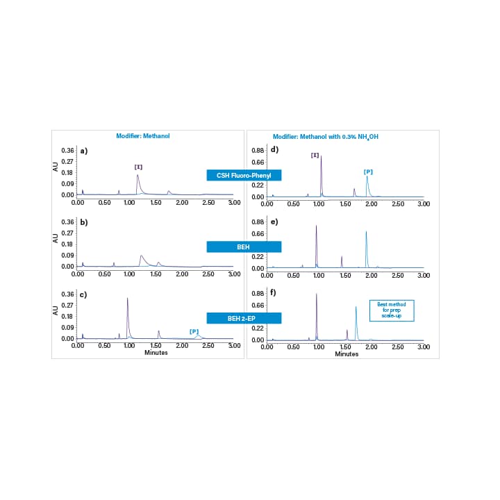
Figure 39. Initial column screening experiments using methanol (left) and methanol with 0.3% NH4OH (right) as the co-solvent. The columns were 2.1x50 mm ACQUITY UPC2 columns with 1.7 µm particles. The screening gradient was from 4–40% in 2 minutes at a flow rate of 1.5 mL/min. The temperature was 40°C and the back pressure was set to 1800 psi.
To optimize the separation for scale-up, focused gradients were developed for the intermediate and product separately. The co-solvent concentration at elution was calculated based on the slope of the screening gradient and the retention time for each peak of interest. The intermediate eluted at 14% co-solvent while the product eluted at 29% co-solvent. 2-minute focused gradients were developed centered on those percentages; starting 5% lower and ending 5% higher (Figure 40).
For scale-up the same column chemistry was used and the ratio of length to particle size (L/dp) was kept constant. The 3 x 50 mm analytical column with 1.7 µm particles (L/dp = 29.4) scaled to the 19 x 150 mm prep column with 5 µm particles (L/dp = 30). The scaled chromatography (focused), and mass directed collection is displayed in Figure 41. Figure 42 shows analysis of the Imatinib product and intermediate fractions.
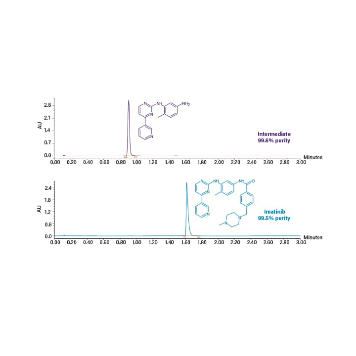
Figure 41. Scaled-up preparative chromatography with mass directed collection of the intermediate (top) and product (bottom). The separations used methanol with 0.3% NH4OH as co-solvent and the gradients were 5.1 minutes. Focused gradients of 9–19% co-solvent and 24–34% co-solvent were used for the intermediate and product purification respectively.
Figure 42. Fraction analysis of the intermediate (top) and Imatinib product (bottom). Initial analytical screening parameters were used with a co-solvent gradient of 4–40% in 2 minutes.