Bands, Peaks and Band Spreading
How a Chromatographic Band is Formed
A sample mixture is transferred from a sample vial into a moving fluidic stream [mobile phase]. The sample is then carried by the mobile phase to the head of a chromatographic column by a high pressure pump. The mobile phase and injected sample mixture enters the column, passes through the particle bed, and exits, transferring the separated mixture to a detector [Figure 3].
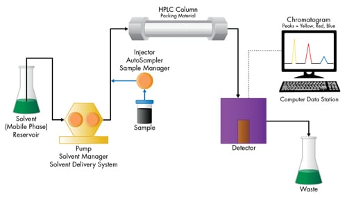
Figure 3: Representation of an HPLC system.
First, let’s consider how the sample band is separated into individual analyte bands [flow direction is represented by green arrows]. Figure 4A represents the column at time zero [the moment of injection], when the sample enters the column and begins to form a band. The sample shown here, a mixture of yellow, red, and blue dyes, appears at the inlet of the column as a single black band.
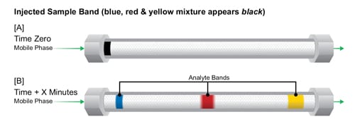
Figure 4: Understanding how a chromatographic column works – analyte bands.
After a few minutes, during which mobile phase flows continuously and steadily through the packing material particles, we can see that the individual dyes have moved in separate bands at different speeds [Figure 4B]. This is because there is a competition between the mobile phase and the stationary phase for attracting each of the dyes or analytes. Notice that the yellow dye band moves the fastest and is about to exit the column. The yellow dye has a greater affinity for [is attracted to] the mobile phase more than the other dyes. Therefore, it moves at a faster speed, closer to that of the mobile phase. The blue dye band has a greater affinity for the packing material more than the mobile phase. Its stronger attraction to the particles causes it to move significantly slower. In other words, it is the most retained compound in this sample mixture. The red dye band has an intermediate attraction for the mobile phase and therefore moves at an intermediate speed through the column. Since each dye band moves at a different speed, we are able to separate the mixture chromatographically.
How a Chromatographic Band Becomes a Peak
Each specific analyte band is made up of many analyte molecules. The center of the band contains the highest concentration of analyte molecules; while the leading and trailing edges of the band are decreasingly less concentrated as they interface with the mobile phase [Figure 5].

Figure 5: Concentration profile of green analyte molecules within the analyte band.
As the separated dye bands leave the column, they pass immediately into a detector. The detector sees [detects] each separated compound band against a background of mobile phase [see Figure 6]. An appropriate detector [UV, ELS, fluorescence, mass…etc.] has the ability to sense the presence of a compound and send its corresponding electrical signal to a computer data station where it is recorded as a peak. The detector responds to the varying concentration of the specific analyte molecules within the band, where the center of the band [highest population of analyte molecules] is interpreted by the detector as the apex of the peak.
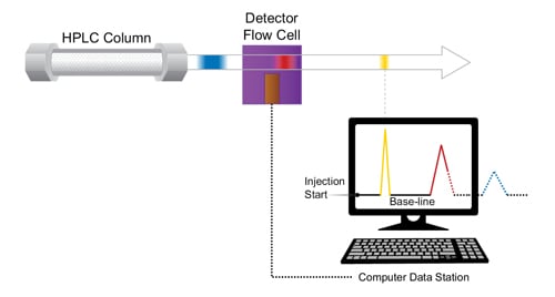
Figure 6: Peaks are digitally created as an electronic response to the analyte band as it passes through the detector.
What Is a Chromatogram?
A chromatogram is a representation of the separation that has chemically [chromatographically] occurred in the HPLC system. A series of peaks rising from a baseline is drawn on a time axis. Each peak represents the detector response for a different compound. The chromatogram is plotted by the computer data station [see Figure 6]. The yellow band has completely passed through the detector flow cell; the electrical signal generated has been sent to the computer data station. The resulting chromatogram has begun to appear on the screen. Note that the chromatogram begins when the sample is first injected and starts as a straight line set near the bottom of the screen. This is called the baseline; it represents pure mobile phase passing through the flow cell over time. As the yellow analyte band passes through the flow cell, a signal [which varies depending on the concentration of the analyte molecules] is sent to the computer. The line curves, first upward, and then downward, in proportion to the concentration of the yellow dye in the sample band. This creates a peak in the chromatogram. After the yellow band passes completely out of the detector cell, the signal level returns to the baseline; the flow cell now has, once again, only pure mobile phase in it. Since the yellow band moves fastest, eluting first from the column, it is the first peak drawn. A little while later, the red band reaches the flow cell. The signal rises up from the baseline as the red band first enters the cell, and the peak representing the red band begins to be drawn. In this diagram, the red band has not fully passed through the flow cell. The diagram shows what the red band/peak would look like if we stopped the process at this moment. Since most of the red band has passed through the cell, most of the peak has been drawn, as shown by the solid line. If we would continue the chromatographic process, the red band would completely pass through the flow cell and the red peak would be completed [dotted line]. The blue band, the most strongly retained, travels at the slowest rate and elutes after the red band. The dotted line shows you how the completed chromatogram would appear if we had let the run continue to its conclusion. It is interesting to note that the width of the blue peak will be the broadest because the width of the blue analyte band, while narrowest on the column, becomes the widest once it leaves the column. This is because it moves more slowly through the chromatographic packing material bed and requires more time [and mobile phase volume] to be eluted completely. Since mobile phase is continuously flowing at a fixed rate, this means that the blue band widens and is more dilute. The detector responds in proportion to the concentration of the band, therefore, the blue peak is lower in height and larger in width.
Band Spreading
Before the sample/analyte band reaches the detector, it will pass through multiple components of the chromatographic system that will contribute to the distortion and broadening of the chromatographic band [Figure 7]. This phenomenon is referred to as band spreading. As the analyte band becomes wider, the resulting chromatographic peak width is increased. The wider band results in a dilution effect that produces a decrease in peak height accompanied by a loss in sensitivity and resolution. Conversely, if band spreading is minimized, narrower chromatographic bands are achieved, resulting in higher efficiency. These taller, narrower chromatographic peaks are easier for the detector to see, allowing for higher sensitivity and resolution due to a more concentrated analyte band. It is therefore important to be aware of the factors that influence band spreading in efforts to reduce and control those influences to improve overall chromatographic performance.
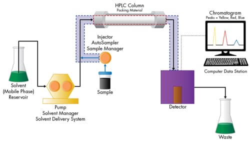
Figure 7: Band spreading will occur along the flow path from the injector (sample band), into, through and out of the column (analyte bands), and then into the detector.
Within a chromatographic system, both column and extra-column [everything outside the column] influences contribute to band spreading. Extra-column sources include the injection volume, the fluidic path of the instrument between the sample injector and the column, and from the exit of the column to the detector [including the flow cell] and all connections included therein. Column sources of band spreading include the particle size of the packing material, how well the material within the column is packed and its diffusion characteristics in relation to the speed of the mobile phase, analyte size and geometry. The summation of the variances (σ2) for each one of these contributors impacts the width of a peak [Figure 8].

Figure 8: As a statistical function, plate count can be thought of as the population variance [σ2], which is a summation of both extra-column and column variances. The population variance [σ2] measures the narrowness of a Gaussian peak [σ] relative to its elution volume.
In order to achieve significantly improved performance in liquid chromatography, a reduction in both extra-column and column band spreading influences is necessary. The ACQUITY UPLC System is based on the concept of reducing both forms of band spreading such that gainful improvements in efficiency and sensitivity can be reached [Figure 9].
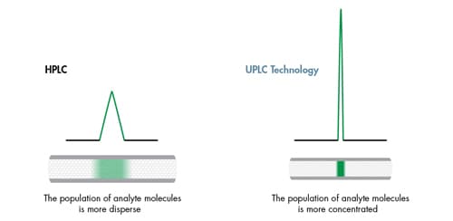
Figure 9: Impact of system band spreading [column and extra-column] on peak shape.
Addressing Extra-column [Instrument] Band Spreading
To realize a significant improvement in chromatographic performance, a substantial engineering effort was undertaken to design an LC instrument that could accommodate the pressures produced by small particle [sub-2 µm] packings, while minimizing the dispersion of the flow path such that theoretical performance of the separation column could be achieved. It is equally important that the instrument is a reliable, robust and precise analytical tool for routine laboratory use. To demonstrate the importance of instrument design, one needs to understand how system dispersion [instrument + column band spreading] can impact chromatographic results.
The measurement of plate count [N], or efficiency, takes into account the dispersion of a peak. The width of a peak is directly related to how wide the analyte band is as it passes through the detector, while the apex of that peak is the point at which the greatest concentration of analyte molecules exists within that band. This measurement is performed under isocratic conditions.
The plate count equation can be derived as shown in Figure 10, where [Vn] is the elution volume of the peak, [w] is peak width, and [a] is a constant that is determined based on the peak height at which the width of the peak is measured. Each method of measuring peak width will yield identical plate count results, as long as the peak is perfectly symmetrical. If the peak exhibits any fronting or tailing, these methods of measurement will yield different results.
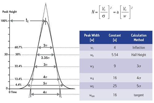
Figure 10: Equation for determining plate count. The narrower the peak width [w], the higher the plate count.
It is a common misconception that plate count refers only to the performance achieved by the column itself. However, the band spreading from both the column and the instrument also influence the peak width from which the plate count is determined. To demonstrate the influence of the instrument itself on band spreading, a single HPLC column was run on two different instruments; a standard HPLC [band spread = 7.2 µL] and an ACQUITY UPLC System [band spread = 2.8 µL]. Since the same column is run on both systems, the band spreading contribution of the column is held constant. The increase in efficiency observed on the ACQUITY UPLC System demonstrates how an instrument with less band spreading will generate narrower peak widths, resulting in a higher plate count [Figure 11].
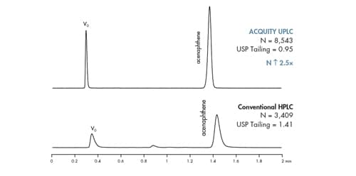
Figure 11: The significant impact of instrument band spreading on column performance. The same column was run on an ACQUITY UPLC System and a conventional HPLC system. [ACQUITY UPLC BEH C18 2.1 x 50 mm, 1.7 µm column; flow rate = 0.4 mL/min.]
The Influence of Tubing Length and Diameter
After the sample band is introduced into the fluidic stream, it travels to the column. The ACQUITY UPLC Sample Manager was designed to minimize the distance between the injector and column inlet in order to minimize band spreading. The column separates the sample band into individual analyte bands. Then the chromatographically separated analyte bands are transferred from the column to the detector. At first glance, one may not consider the importance of the internal diameter [ID] of the tubing connecting the column outlet and detector inlet. However, the internal diameter can greatly impact instrument band spreading [Figure 12].
As one may expect, band spreading will decrease with decreasing tubing ID. By flowing a concentrated analyte band into a large ID tube, the band will become much less concentrated resulting in a wider, distorted peak and decreased sensitivity. Additionally, friction along the walls of the tubing will cause analyte molecules in contact with the tubing walls to move slower than molecules in the center of the tube, resulting in a distorted band profile. The distance between the center and the outer edges of the analyte band become less as tubing ID decreases. This reduces the amount of distortion in the band. It is equally important to minimize the length of tubing, as excessive lengths can also distort a sample band.
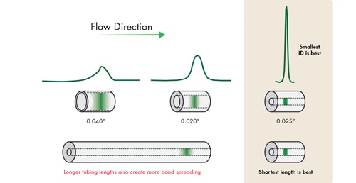
Figure 12: Analyte band spreading as a function of tubing ID and length.
The Impact of Detector Settings on Extra-column Band Spreading
In addition to fluidic-based band spreading contributions of the instrument, digital detector settings related to acquisition speed and filter constant also influence the chromatographic result. This is especially important for UPLC applications, since peak widths are often very narrow [1–2 seconds wide], and analysis time can be very short. When setting the acquisition speed of the detector, the selection should be based upon acquiring sufficient data points across a peak to properly represent the peak. Setting the detector rate too high will negatively impact the signal-to-noise ratio causing the baseline noise to increase without an increase in the signal height of the analyte of interest. Conversely, setting the detector acquisition rate too slow will result in inadequate data points across the peak, thus reducing the observed chromatographic efficiency and compromising the ability to reproducibly perform quantitation. In addition, a time constant [digital filter] is used to smooth out data points to optimize signal-to-noise and can be used conjointly with or independent from, the acquisition speed.
Detector settings become increasingly more important as the width of the analyte band narrows. This requires an acquisition speed that is not only fast enough to digitally create a peak of that speed, but also to properly render the high resolution separation achieved in the UPLC column, if closely eluting peaks exist.
At slower flow rates when peaks are more disperse in time, these settings are more forgiving. However, as the peaks become narrower and the analysis more rapid [as in UPLC separations], a judicious setting of acquisition speed and time constant must be maintained [Figure 13]. When using UPLC Technology for ‘real-life’ applications, it is wise to select the detector data acquisition rate [Hz] that accurately captures the peak shape of the narrowest peak, and then apply a filter time constant [seconds] that gives optimal signal-to-noise and resolution for the analysis.
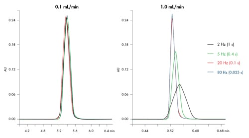
Figure 13: Impact of acquisition speed [Hz] and time constant[s] on peak formation. UPLC peak widths can be very small [1–2 seconds wide]. Therefore, it is critical that proper detector settings are used. Probe is acenapthene analyzed isocratically on an ACQUITY UPLC BEH C18 2.1 x 50 mm, 1.7 µm column; mobile phase 65/35 ACN/H2O; ACQUITY UPLC System.