METHOD SCALE-UP
When there is initial demonstration of an isolate’s potential value, a separation method can be “scaled-up” to generate increasing quantities of that isolate for further evaluation. Small scale separation attributes such as resolution can be easily maintained at large scale. Flow rate, sample load and system hardware must be modified to effectively transfer the separation to higher capacity columns through defined mathematical formulas.
The first stage of scale-up will usually encompass the production of mg to gram quantities of isolate for various uses ranging from early biological evaluation to establishment of structure-activity relationships for product analogs with improved therapeutic properties. Further stages of scale-up involve material quantities from 100 g to multiple kilograms and beyond for preclinical and clinical development, which if successful will ultimately culminate in full scale manufacturing. At this scale documentation and quality controls such as Good Manufacturing Practices (cGMP) come into play.¹
|
Purification Scale
|
Target Amount
|
Typical Application
|
|
Analytical micro-purification
|
µg
|
Isolation of enzymes or compounds used in small scale drug discovery experiments
|
|
Semi-Prep
|
mg
|
Small scale biological testing Structure elucidation and characterization of metabolites
|
|
Prep
|
g
|
Analytical reference standards Toxicology scouting studies
|
|
Process
|
kg
|
Industrial scale drug and active compound manufacturing
|
Table 3: Chromatographic scale, target amount and associated application.
The scale-up workflow is a step-wise process. Scale-up calculations must be performed accurately, or else the end result may not provide the resolution achieved in the small scale separation. To increase the success of method scaling and, maintain retention time and selectivity, several requirements need to be closely considered:
■ Identical mobile phase must be used at small and large scale.
■ Columns of identical column chemistry, length and particle size provide easiest scale up (Alternatively, the particle size can be changed as long as the, L/dp, column-length-to-particle-size ratio of the initial method is maintained).
■ Samples need to be prepared at the same concentration, in the same diluent.
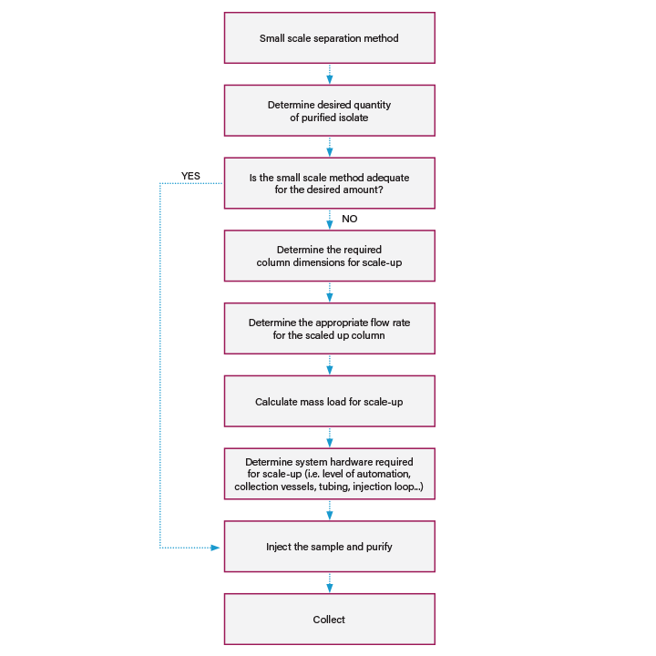
Figure 18: Scale-up workflow
DWELL VOLUME DETERMINATION
Dwell volume (delay volume, system volume) is important for preserving peak resolution of early eluting peaks when scaling up or changing systems. It is defined as the volume from the point of gradient formation to the head of the column. For high-pressure- mixing LC systems this volume primarily comprises of the mixer, connecting tubing, and autosampler loop. Low-pressure mixing systems combine the solvents upstream from the pump, so additional tubing plus the volume of the pump head (or heads) plus the mixer, connecting tubing, and autosampler loop contribute to the overall dwell volume.
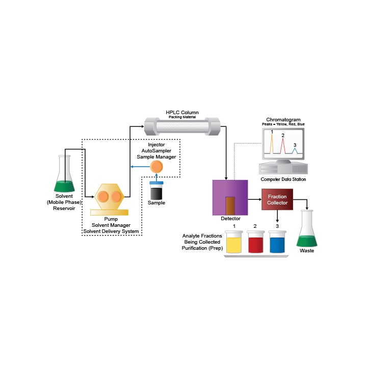
Figure 19: Purification flow path components that contribute to dwell volume are circled (dashed line).
When mobile phase components are mixed on-line for isocratic separations, the dwell volume still exists, but since the mobile phase concentration is constant, there is no observable difference in chromatography. Gradient methods on the other hand, rely on a change in the concentration of mobile phase over time to generate peak separation. Compensation for the dwell volume in a gradient method ensures peak retention times are maintained, especially important when the intent is to collect purified fractions.
To determine the dwell volume, a step gradient of mobile phase A and the mobile phase B solvents containing an additive with different UV absorption (e.g. 0.05 mg/mL uracil, or 0.2% acetone in acetonitrile) can be used according to the method found at www.waters.com/prepcalculator in the “Analytical to Prep Gradient Calculator.”
- Remove the column.
- Use acetonitrile as mobile phase A, and acetonitrile with additive (0.05 mg/mL uracil, or 0.2% acetone) as mobile phase B.
- Set UV detector at 254 nm.
- Calculate the dwell twice (i.e. Calculate dwell volume for the flow rate in the original instrument, and for the intended flow rate with the target instrument.)
- Collect the baseline at 100% A for 5 minutes.
- Program a step change at 5 minutes to 100% B, and collect data for an additional 5 minutes.
- Measure absorbance difference between 100% A and 100% B.
- Measure the time at 50% of that absorbance difference.
- Calculate the time difference between start of the step and the 50% point.
- Multiply the time difference by flow rate.
|
| |
| |
| |
| |
| |
| |
| |
| |
| |
Table 4: Procedure for the determination of dwell volume.
CAPACITY
In purification chromatography, maintaining adequate resolution for the compound intended for collection is the primary focus. Column capacity, or load, is gauged by the resolution of the compound and neighboring peaks. Although column capacity is influenced primarily by column length and diameter, other factors such solubility and the complexity of the sample mixture can make a contribution. The capacity trends are as follows:
■ Capacity depends primarily on solubility of the particular sample.
■ Capacity is higher for simple mixtures.
■ Capacity is lower where high resolution is required.
■ Capacity is dependent on loading conditions.
|
|
|
|
Diameter (mm)
|
|
|
|
Length (mm)
|
4.6
|
10
|
19
|
30
|
50
|
|
50
|
3
|
15
|
45
|
110
|
310
|
|
75
|
—
|
—
|
—
|
165
|
—
|
|
100
|
5
|
25
|
90
|
225
|
620
|
|
150
|
8
|
40
|
135
|
335
|
930
|
|
250
|
13
|
60
|
225
|
560
|
1550
|
|
|
|
|
|
|
|
|
Reasonable flow rate (mL/min)
|
1.4
|
6.6
|
24
|
60
|
164
|
|
Reasonable injection volume (µL)
|
20
|
100
|
350
|
880
|
2450
|
Table 5: Estimated loading capacity (mg) for common prep column dimensions. Example: For the 4.6 x 50 mm column, the predicted load is 3 mg per 20 µL injection.
Capacity for a specific compound of interest is determined before method scale-up through loading studies. These studies are performed at small scale and are executed by one of the following techniques; a sample is prepared at a high concentration and the injection volume incrementally increased, or a sample is prepared at multiple concentrations and the injection volume held constant. For either technique, the goal is to determine the maximum concentration or injection volume that maintains adequate resolution of the compound of interest from surrounding impurities. Once the column capacity is determined, it can be scaled-up using a formula for larger diameter columns and workflows.
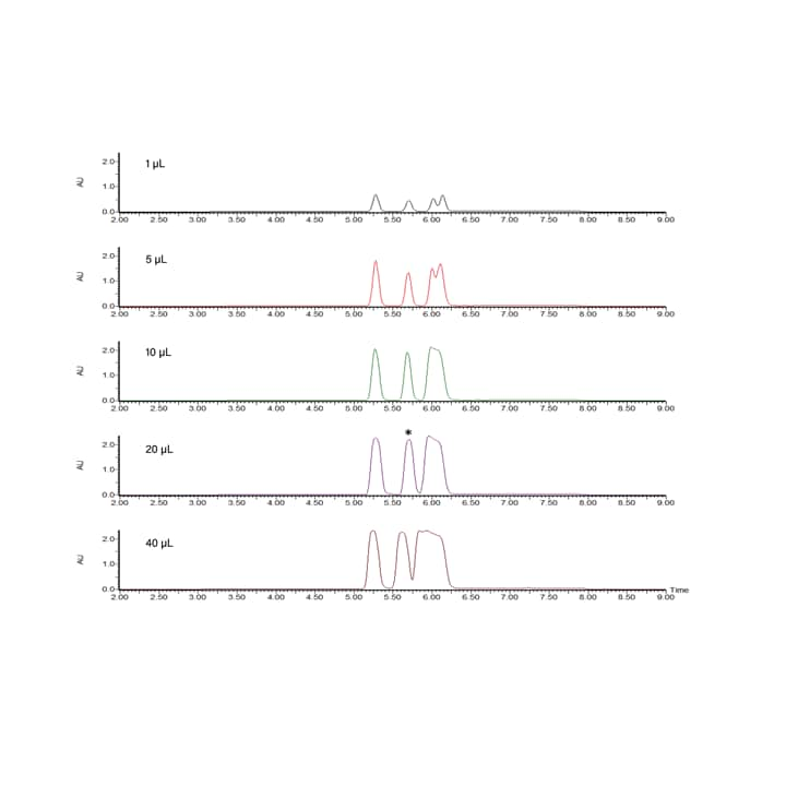
Figure 21: Volume loading study. Note the decrease in resolution as the load for the peak with the asterisk increases.
Equation 10: Concentration load scale-up
Therefore, to scale-up an 1800 µg (1.8mg) load on a 4.6 mm x 50 mm analytical column to the equivalent load on a 19 mm x 50 mm prep column:
Equation 11: Injection volume scale-up
To scale up a 20 µL injection volume load:
At-Column-Dilution
Strong solvents such as DMSO can improve sample solubility resulting in a potential increase in column capacity. Unfortunately, large injection volumes of strong solvents can distort chromatography resulting in a reduction rather than an increase in amount of product that can be successfully isolated.
Distortion occurs when strong solvent is carried from the injector to the head of the column as a plug sandwiched in a stream of aqueous solvent. Sample precipitation can occur at the edges of the plug where the strong sample solvent is diluted with the aqueous solvent. This precipitation can result in a blockage in the fluid path and lead to a high-pressure system shutdown.
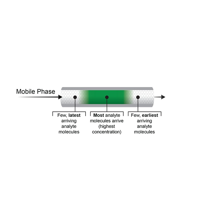
Figure 22: Dilution of the sample plug with mobile phase inside the column. Precipitation may occur at the edges of the sample plug as it travels through a column containing aqueous mobile phase if the sample is prepared in strong diluent.
If precipitation does not cause a system shutdown, the sample enters the column, but there is no retention until the sample plug is diluted with mobile phase. With larger injections, the volume required to dilute the sample can only be derived by moving the plug a substantial distance along the column. In such cases, the sample is deposited as a broad band that occupies a large fraction of the column volume. The result is incomplete peak resolution of peaks spread over large volumes of eluent. This situation may be reduced by strictly limiting both the volume and mass of sample injected.
The alternative is substantial dilution of the sample with water, or weak solvent, to ensure adequate retention.
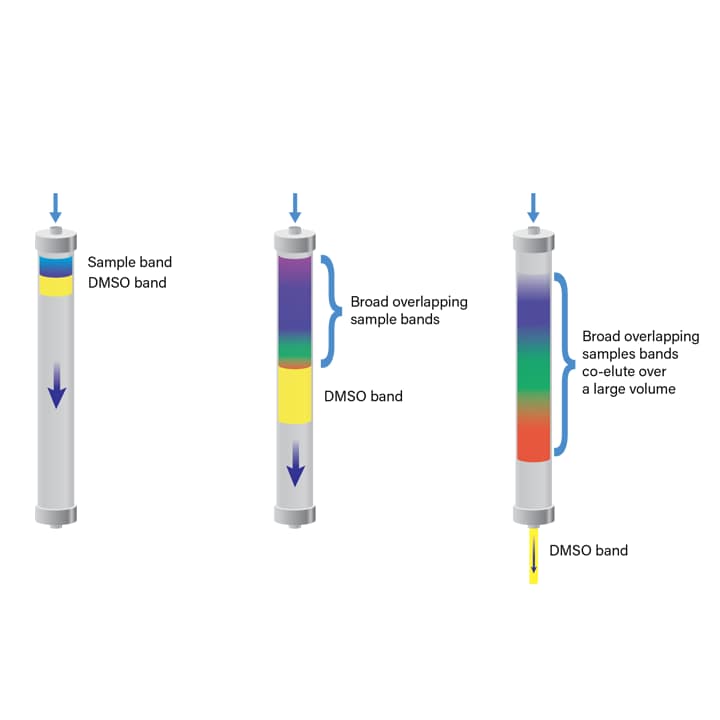
Figure 23: Conventional approach for injection of samples in strong solvent. The sample plug is diluted as it moves along the column resulting in distortion of the peaks.
Neither approach is completely satisfactory as throughput and recovery are compromised. Alternatively, in an At-Column-Dilution system, the system is reconfigured so that the sample plug is carried to the entrance of the column, where it is continuously diluted with a stream of aqueous diluent. The rate of transfer into the column is so high that precipitation cannot occur. The sample molecules are then adsorbed to the packing material as very narrow bands that can be eluted as well-resolved, small-volume peaks. System ruggedness is improved with At-Column-Dilution since the sample has limited ability to precipitate in the loop or at the column head.
Improved resolution between sample component peaks permits increasing the sample size and thereby reducing the number of injections required for isolation. In practice, with At-Column-Dilution, the column loading can often be increased by three to five fold. The incidence of high-pressure shutdowns is reduced and column lifetime is extended.
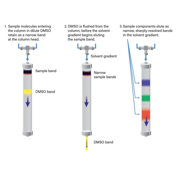
Figure 24: At-Column-Dilution system. The sample plug is carried to the entrance of the column, where it is continuously diluted with a stream of aqueous diluent and precipitation does not occur. The sample bands elute as well-resolved, small-volume peaks.⁶
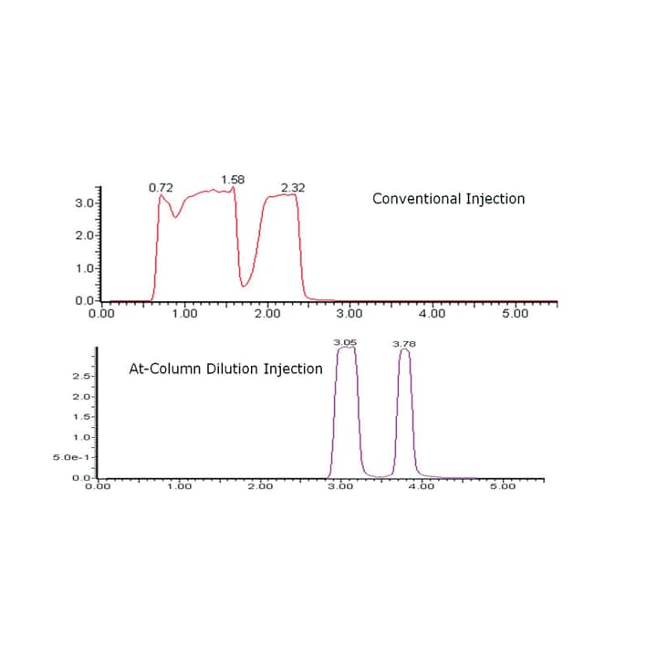
Figure 25: Comparison of a sample dissolved in strong solvent using conventional injection and injection by At-Column-Dilution. 1000 µL to equal 133 mg on column were injected.³
FLOW RATE SCALE-UP
To successfully maintain separation quality during scale-up, the linear velocity must remain constant between small and large scale columns therefore flow rate scaling works best between large and small scale columns of the same length, particle size and packing material. Capabilities of the system hardware such as maximum pump flow and backpressure limits must be considered when scaling the flow rate. If the hardware does not meet the flow rate requirements, appropriate instrumentation changes should be considered to meet the scale.
Equation 12: Flow rate scale-up
For example, if the flow rate for an analytical column (5 µm, 4.6 mm x 50 mm) is 1.5 mL/min the flow rate on a prep column (5 µm, 19 mm x 50 mm) column is calculated:
GRADIENT DURATION SCALE-UP
Typically, no gradient change is required during scale-up if the flow rate is adjusted to maintain the linear velocity of the mobile phase. If column lengths are different, the
gradient time must be calculated to maintain the separation and retention time obtained at small scale.
Equation 13: Gradient time scale-up
For example, a linear gradient segment that that lasts 5 minutes on a 50 mm analytical column will be 10 minutes on a 100 mm prep column:
PREP CALCULATOR
Mass, flow and gradient scale-up calculations can also be performed within the Prep OBD Columns Calculator. The calculator is an easy to use application that aids in all analytical-to-prep scaling calculations including mass load, system volume, flow rates, solvent volume consumption, split flow ratios for mass spectrometer driven chromatography, and focused gradient UPLC methods to preparative methods transfer. The application can be accessed at www.waters.com/prepcalculator or though Waters based purification software such as ChromScope.™
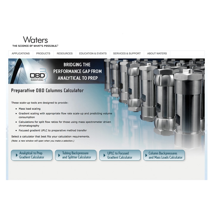
Figure 26: Waters Prep OBD Column Calculator available in the Web Toolbox at www.waters.com/prepcalculator.
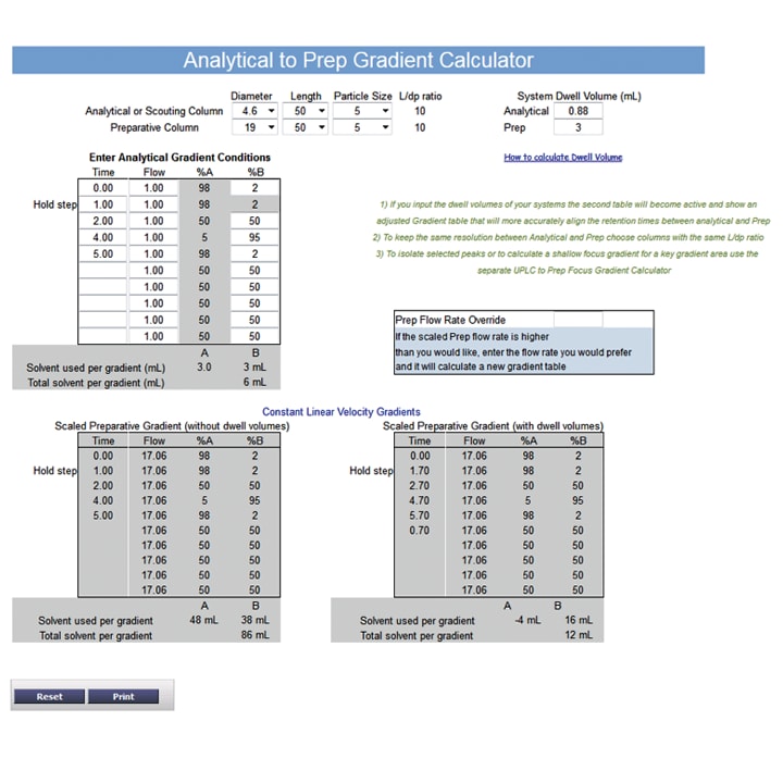
Figure 27: The Waters Analytical to Prep Gradient Calculator determines the prep conditions from the analytical separation.