Scouting Gradients

SCOUTING

Although complex separations are most impacted by the selectivity of the column packing material, it is most efficient when developing a separation method targeted for purification to begin with optimization of the sample separation generated with a rapid scouting gradient. The goal of the scouting gradients is to determine the approximate solvent concentration required to elute the compound(s) of interest from the column. Scouting gradients typically start from the same strong solvent concentration (2–10%) and linearly increase to 25%, 75%, 50%, and 90–95%.

Table 1: Example of rapid linear gradient scouting study.

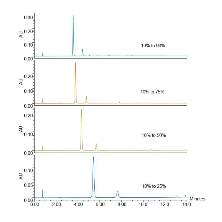
Figure 4: Rapid scouting gradients. Resolution becomes higher as the gradient slope decreases.²

Upon completion of the scouting gradients, the results are reviewed and evaluated by a series of questions before moving to the next step:

■ Does the rapid scouting gradient provide adequate separation for the compound of interest?

■ Is the rapid scouting gradient adequate for speed or efficiency?

■ Can the separation of the compound of interest from other peaks be maintained at the sample load required?

I the scouting gradient does not yield an adequate result, it can be optimized through method focusing, or as an alternative, the separation can be modified entirely through pH, solvent or other chromatographic variables.

OPTIMIZING THE METHOD

The scouting run that provides the greatest resolution for the compound of interest can be optimized by modifying the composition of strong and weak solvents. The composition can either remain constant (isocratic), or it can change per a given unit time or column volume (gradient).

Isocratic Elution

In an isocratic separation, weak solvent and strong solvent are maintained in an unchanging ratio per unit time. Isocratic solvent can be prepared offline by the analyst, or mixed online with a HPLC pump capable of proportioning the different solvents at a consistent, predetermined rate. This elution mode is convenient, consistent and robust because retention time influences caused by dwell volume are negligible when transferring a method between systems.

Isocratic elution has drawbacks and may not be appropriate for all separations. There are inherent issues including poor resolution of early eluting peaks, decreased symmetry due to peak tailing, decreased sensitivity due to band broadening, and problems with column contamination due to the buildup of strongly retained compounds.

Gradient Elution

Gradient separations in reversed-phase or ion exchange usually involve on-line mixing of mobile phase to achieve a steady increase in the organic solvent over the course of the analysis. At the beginning of the gradient when the solvent strength is low the analyte is partitioned in the stationary phase or remains at the head of the column. As the solvent strength increases, the analyte is transferred to the mobile phase, moves along the column, and finally is eluted.

Gradient elution provides the ability to separate analytes with a wide range of hydrophobicity in a reasonable time frame. Additional advantages can include improved peak resolution and increased sensitivity due to greater peak height. Column deterioration is also minimized when strongly retained components are washed from the column at the end of the run.

There are also disadvantages when using gradient elution. Consistent, pulse free online gradient mixing is required therefore expensive pump instrumentation is often necessary. Additionally, precipitation can occur when some mobile phases are mixed in certain combinations. Run times can be long due to post gradient

re-equilibration, and instruments can vary in dwell time (Vd) causing method transfer issues, without adequate compensation.

Linear Gradient

Linear gradients progress with a constant increase in the composition of strong solvent throughout the entire run. They are often used in rapid screening experiments to quickly determine the solvent ratio that elutes the peak of interest and keep run time reasonably short, which results in elution in less time with less time and reduced solvent cost.

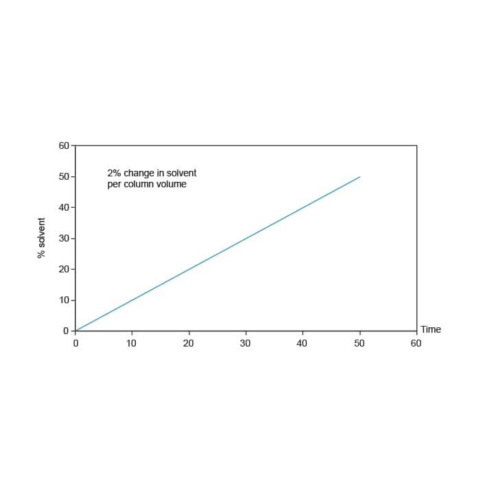
Figure 5: Solvent profile for a linear gradient.

Segmented Gradient

A segmented gradient is a combination of a series of linear gradients, each with a different slope or steepness. The shallow segments resolve the compounds of interest, while the steep segments are areas of the chromatogram where high resolution is not required, such as in a post separation wash.

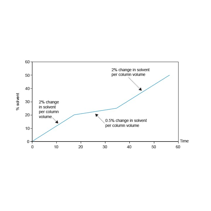
Figure 6: Solvent profile for a segmented gradient.

Focused gradients are typically shorter and more exaggerated than in segmented gradients. Generally, the solvent strength is very low immediately after injection. It is then rapidly increased to between 2–5% below the solvent ratio required for elution of the compound of interest (i.e. 22% elution concentration – 2% = 20% start shallow gradient). A shallow gradient then proceeds at about 1/5 the slope determined in the rapid scouting separation to finally end between 2–5% above the elution concentration for the compound of interest (i.e. 22% + 2% = 24% stop shallow gradient). Finally, the percentage of solvent is quickly increased to wash the column of any remaining sample components.

Developing a Focused Gradient

The following calculations can be used to generate a focused gradient for the compound of interest after the sample has been analyzed with a rapid scouting gradient. Each equation is followed by a theoretical example.

First, the system dwell volume must be determined for the instrument that was used for the scouting gradient run. Instructions for dwell volume determination can be found in the section of this primer titled "Dwell Volume Determination" or it can be found in the “Analytical to Prep Gradient Calculator” application tool at www.waters.com/prepcalculator.

Additionally, column volume must also be determined for the column employed for the scouting run. It can be calculated by using the volume of a cylinder V = πr²h and the compensating for the volume occupied by packing material i.e. V = πr²h (66%). The “Analytical to Prep Gradient Calculator” application tool can also be used to perform this calculation.

Equation 1: Column volume

Example:

Equation 2: Offset volume between gradient formation and the detector

*System volume or Dwell volume

Example:

Equation 3: Time to detector

Equation 4: Time when elution concentration was formed

Example:

Equation 5: Percent elution concentration

Example:

Equation 6: Number of column volumes (CV)

Example:

Equation 7: Scouting gradient slope

Example:

Equation 8: Focused gradient slope

Example:

The focused gradient segment is created from 5% below, to 3–5% above the estimated elution percentage. As an example, the elution percentage is 79%.

Equation 9: Length of time for the focused gradient segment

Example:

The last step is to write the focused gradient using the values calculated in the previous formulas.

Scouting gradient:

Focused gradient: