The Promise of Small Particles
The Relationship between Resolution and Intra-column Band Spreading
If we think about chromatographic resolution in the most basic sense, it is simply the width [w] of two peaks relative to the distance [tR,2 – tR,1] between those peaks. If we can make those peaks narrower or further apart, we can improve resolution.

Figure 14: Fundamental resolution equation. [N] is plate count, [α] is selectivity and [k] is retention factor.
Resolution can be expressed mathematically in more relevant terms in the form of the fundamental resolution equation. The resolution equation is comprised of physical and chemical parameters that affect chromatographic resolution; efficiency [N], selectivity [α] and retentivity [k]. Selectivity and retentivity are chemical factors that have historically been easier to manipulate to improve resolution. These parameters can be affected by changes such as temperature, elution solvent, mobile-phase composition and column chemistry. Efficiency is a physical [mechanical] parameter that is more difficult to manipulate due to its square root influence on resolution. However, efficiency can have a significant impact on resolution if the particle size is very small. UPLC Technology focuses on improving resolution by utilizing sub-2 µm particles to improve system efficiency.
It is easier to understand how these parameters affect resolution if we think about how these three terms are represented chromatographically [Figure 15]. Retentivity [k] and selectivity [α] are chemical factors that move peaks relative to one another and are a measure of the interaction of the analytes with the stationary phase and the mobile phase. We can improve resolution by increasing k. However, longer retention times, lower sensitivity and wider peak widths result. An increase in α can result in more resolution, the same peak elution order in a similar amount of time, and/or an elution order change. Efficiency [N] is a physical measure of band spreading in a separation. Assuming that N is improved by reducing particle size of the packing material, the center-to-center peak distance does not change. Additionally, a reduction in particle size will result in narrower, more efficient chromatographic peaks, thus improving resolution and sensitivity.
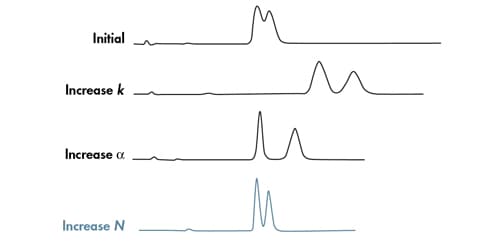
Figure 15: The impact of individual chemical and mechanical factors on resolution.
The Relationship between Resolution, Efficiency and Particle Size
UPLC Technology maximizes the physical [mechanical] contribution to resolution by minimizing instrument band spreading, enabling the use of higher efficiency, smaller particle columns [1.7 µm – 1.8 µm]. With simple chromatographic examples and basic arithmetic, one can gain a better understanding of the chromatographic principles behind UPLC Technology.
As stated in the fundamental resolution equation, resolution is directly proportional to the square root of efficiency.

Figure 16: Resolution [Rs] is directly proportional to the square root of efficiency [N].
Additionally, efficiency is inversely proportional to the particle size. This means, if the particle size of the packing material is decreased, separation efficiency increases. For example, if the particle size of the packing material is reduced from 5 µm to 1.7 µm [3´], theory predicts that efficiency should increase 3´, resulting in a 1.7´ increase in resolution [square root of 3].

Figure 17: At constant column length, efficiency [N] is inversely proportional to particle size [dp].
In order to achieve the gains of efficiency and resolution predicted by theory, the optimal flow rate must be run with respect to the particle size. The optimal flow rate [Fopt] is inversely proportional to the particle size. This means, if the particle size is reduced from 5 µm to 1.7 µm [3´], the optimal flow rate in which to run that particle increases 3´, resulting in a reduction in analysis time to the same degree [3´], therefore increasing sample throughput.

Figure 18: At constant column length, flow rate [Fopt] is inversely proportional to particle size [dp], resulting in a reduction of analysis time [T] proportional to the reduction in particle size.
One of the first things we observe as chromatographers is what happens when the chromatographic flow rate is changed. If the flow rate is increased, analytical run time decreases. Additionally, the width of the peak also decreases. As peak width becomes narrower, the height of that peak increases proportionally. Narrower peaks that are taller, are easier to detect and differentiate from baseline noise [higher S/N], resulting in higher sensitivity.

Figure 19: Narrower peak widths produce higher efficiency and peak heights. Efficiency [N] is inversely proportional to the peak width [w] squared. Further, as the peak width decreases, the peak height increases proportionally.
These theoretical principles were applied chromatographically. As observed in Figure 20, when extra-column band spreading is minimized as in the ACQUITY UPLC Instrument, the theoretical performance of a column can be achieved.
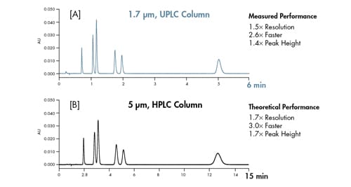
Figure 20: Matching theory to reality. Separations were performed on two columns with same dimensions [2.1 x 50 mm]. Identical chromatographic conditions were used in both separations with the exception of flow rate, which were scaled based on particle size.
The discussion above demonstrates the importance of intra-column band spreading. If one can further understand what processes influence band spreading and how to reduce it, improvements in efficiency, and therefore resolution, can be achieved.
Understanding van Deemter Curves
As described earlier, the width of a peak can be thought of as a statistical distribution of the analyte molecules [variance, σ2]. The peak width increases linearly in proportion to the distance in which that peak has traveled. The relationship between peak width and the distance in which that peak has traveled, is a concept called the height equivalent to a theoretical plate [HETP or H]. Originating from distillation theory, H is a measurement of column performance that takes into account several band spreading related processes. To put this into terms that may be more familiar, the smaller the HETP, the more plates [N] there are in a column [Figure 21].

Figure 21: Simplified equation to determine HETP. [L] is column length, [N] is plate count and [HETP] is height equivalent to a theoretical plate.
If we think about what is occurring at a molecular level within a column [how the analyte molecules are interacting with the mobile phase and stationary phase], we can further understand the different diffusion-related processes that are occurring that contribute to chromatographic performance [Figure 22].
There are several diffusion-related processes occurring simultaneously:
- Analyte molecules are transported to the surface of the particle and around that particle [eddy diffusion]
- Analyte molecules are diffusing back and forth in the bulk mobile phase [longitudinal diffusion]
- Analyte molecules are diffusing into and out of the chromatographic pores [mass transfer].
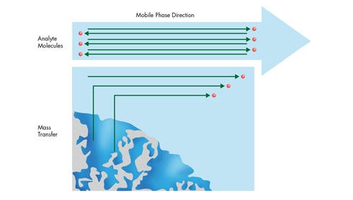
Figure 22: Diffusion-related processes occurring within the column.
These diffusion-related processes can be expressed mathematically in the form of the van Deemter equation.

Figure 23: van Deemter equation.
The van Deemter equation is comprised of three terms:
- The A term [eddy diffusion] is related primarily to the particle size of the packing material. Its value is also determined by how well the chromatographic bed is packed. It is also related to the uniformity or non-uniformity of the flow to and around a particle.
- The B term [longitudinal diffusion] is related to the diffusion of the analyte in the bulk mobile phase and on the stationary phase and decreases with increasing speed of the mobile phase [linear velocity].
- The C term [mass transfer] is related to both the linear velocity [the speed of the mobile phase] and the square of the particle size. Mass transfer is the interaction of analyte molecules with the internal surface of the stationary phase and their distance of diffusion into and out of the pores of the packing material.
We can observe these terms individually by plotting them on a scale of HETP vs. the linear velocity [u] of the mobile phase [Figure 24].
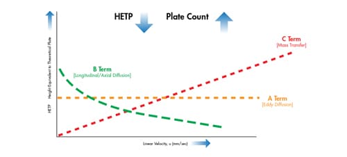
Figure 24: Individually plotted terms of the van Deemter equation.
The A term is plotted as a horizontal line. It is related to the particle size and how well a column is packed and is independent of linear velocity [mobile-phase speed]. As the particle size of the packing material is decreased, the H value also decreases [higher efficiency].
The B term is plotted as a downward sloping curve with increasing linear velocity. This term is independent of the particle size and indicates that if the mobile phase moves at a slower linear velocity, analyte molecules reside in the column for a longer time, and therefore, a greater opportunity exists for band spreading [diffusion] lengthwise within the column. Conversely, if the mobile phase moves at a faster linear velocity, there is less time for diffusion, and therefore there is less time for band spreading to occur.
The C term is plotted as an increasing linear relationship between H and u. Among a distribution of molecules, some molecules enter a stationary-phase pore while others remain in the moving mobile phase until they reach another particle. This is followed by the reverse process, where immobilized molecules detach and move further down the chromatographic bed. It takes time for a molecule to move into and out of the pores, and therefore, as molecules transfer from one particle to the next, the analyte band that contains those molecules broadens as it moves down the length of the column. The smaller the stationary phase particles, the faster this process occurs keeping the analyte band from spreading. If the mobile phase moves fast, a larger distance develops between the immobilized molecules and the ones that move ahead. This indicates that in order for the population of analyte molecules to remain together, the mobile phase should move at a slower linear velocity. As the speed of the mobile phase is increased, the population of analyte molecules will become more disperse, resulting in increased band spreading.
A van Deemter curve is formed upon adding the A, B and C terms together [Figure 25]. Conducting a separation at the linear velocity at which the lowest point in the curve occurs will yield the highest efficiency and therefore, chromatographic resolution.
If we correlate this to the van Deemter equation shown in Figure 23, if particle size is reduced by half, H is reduced by a factor of 2. Hence, it is possible to reduce band spreading within a column by utilizing smaller particles.
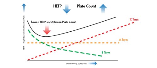
Figure 25: Adding the three individual terms of the van Deemter equation together yields a van Deemter curve.
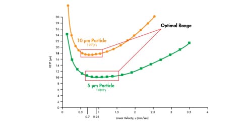
Figure 26: Van Deemter plot comparing 10 µm and 5 µm particles.
For example, Figure 26 depicts a van Deemter plot of a 10 µm particle and a 5 µm particle. As observed on the plot, a large 10 µm particle has a very narrow optimal operating range with respect to linear velocity, to achieve the lowest H value [18 µm @ 0.7 mm/sec]. If the speed of the mobile phase is too slow or too fast, an increase in H [loss of efficiency] is observed, thus reducing chromatographic resolution and sensitivity. However, the 5 µm particle exhibits a much lower H value, [10 µm @ 0.95 mm/sec; higher efficiency] at a higher mobile-phase speed, as well as a larger linear velocity range in which that H value can be achieved. This means, a higher efficiency, and therefore resolution, can be achieved in a faster time than with a column packed with larger 10 µm particles.
To gain additional understanding of this effect, we can further investigate the influence of particle size on the individual terms of the van Deemter equation.
Particle size has a significant impact on the analyte band as it relates to the A term [eddy diffusion]. The path which analyte molecules take to transfer from the bulk mobile phase to the surface of the particle and around that particle takes less time as particle size is decreased. Larger particles cause analyte molecules to travel longer, more indirect paths. The differences in these paths result in different migration times for the analyte molecules within a population, resulting in a broader analyte band and resulting peak. As the particle size of the packing is decreased, the paths of the analyte molecules are encouraged to be more similar in length. This results in narrower analyte bands which translate into narrower peaks, higher efficiency and higher sensitivity [Figure 27].
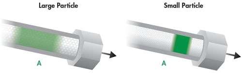
Figure 27: The influence of particle size on the A Term.
Longitudinal diffusion, the B term, is not directly impacted by particle size. However, as particle size decreases, the other parameters of the van Deemter equation, the A and C term, become smaller. Consequently, the optimal linear velocity [mobile-phase speed] increases, resulting in less opportunity for band spreading. Slower linear velocity allows the band of analyte molecules to interact with the packing material for a longer period of time. This means there is more time for axial [lengthwise] diffusion into the mobile phase, resulting in broader, more diffuse analyte bands. At higher linear velocity, the population of analyte molecules is swept through the column in a shorter period of time which enables the analyte band to remain more concentrated, resulting in narrower, higher efficiency peaks due to less time for longitudinal diffusion [Figure 28].
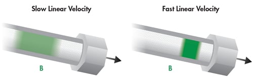
Figure 28: Influence of linear velocity on longitudinal diffusion, the B term.
The C term [mass transfer] is impacted by both linear velocity and particle size. The populations of analyte molecules are transported from the mobile phase to the particle surface. The analyte molecules then move through the mobile phase in the pores to the bonded surface layer (e.g. C18, C8, etc.), interact with the bonded phase and then are swept back out of the pore into the bulk mobile phase. However, the analyte molecules within the population travel into and out of the pore to varying degrees. That means as the molecules return to the bulk mobile phase, the length of the path in which each analyte molecule has traveled is different resulting in a spreading [widening] of the analyte band [Figure 29]. The amount of band spreading that occurs will depend on the speed of the mobile phase [Figure 30].
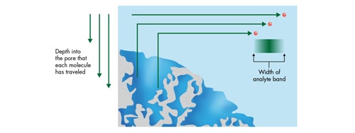
Figure 29: Mass transfer [diffusion] into and out of a chromatographic pore.
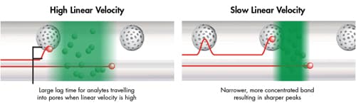
Figure 30: Impact of linear velocity on mass transfer and analyte bands [same particle size].
At a high linear velocity, the time between the molecules interacting with the particle surface and transferring through the mobile phase is longer. The faster the speed of the mobile phase, the quicker the analyte molecules will move through the column, resulting in a broader, less concentrated analyte band. This translates into a broader chromatographic peak and lower sensitivity.
At a slow linear velocity, the length of the steps between interactions to the surface is shorter. This results in a more concentrated analyte band, producing narrower, more efficient chromatographic peaks.
Mass transfer improves dramatically as the particle size is decreased due to its relationship to the square of the particle size [dp2]. For smaller particles, it takes less time for an analyte molecule to travel into the pores, interact with the chromatographic surface, and be swept back into the mobile phase. Therefore, analyte molecules separated on smaller particle columns diffuse much faster, resulting in a sharper, narrower and more efficient chromatographic band [Figure 31].
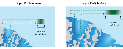
Figure 31: Mass transfer differences related to particle size [representation of a 100Å pore]. Narrower analyte bands are formed with smaller particles.
Reducing particle size will therefore improve mass transfer, thus effectively decreasing the slope of the C term, which leads us to where we are today with UPLC Technology. As can be seen in the van Deemter plot in Figure 32, 1.7 µm particles provide 2-3´ lower HETP values than 3.5 µm particles. Additionally, these lower H values are achieved at a higher linear velocity and over a broader range of velocities. This means that mass transfer is improved dramatically with the smaller particle, enabling better efficiency and resolution. It also means that one can use an increased range of linear velocities to gain this improved performance. Separations are able to be performed at faster linear velocities, thus improving speed of analysis, without compromising resolution.
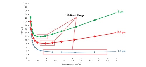
Figure 32: van Deemter plot comparing particle size.
The Impact of Extra-column [Instrument] Band Spreading on van Deemter Plots
As UPLC Technology has gained momentum and popularity in the chromatographic laboratory, van Deemter plots have emerged as a popular method to measure the performance gains of sub-2 µm particles relative to existing HPLC particle sizes. Erroneous conclusions can be made if these comparative measurements are not carried out on instrumentation that minimizes the contribution of extra-column band spreading.
To demonstrate the importance of extra-column band spreading on performance measurement, van Deemter plots were generated on a conventional HPLC instrument [band spread = 7.2 µL], comparing 1.7 µm vs. 2.5 µm particles [Figure 33]. The particle substrate and bonded phase chemistry of the two columns were identical. At first glance, the van Deemter plots infer there is no appreciable difference in the performance of these two columns. How can this be?
In this case, the band spreading of the HPLC instrument results in a similar performance measurement of the 1.7 µm particle UPLC column relative to the 2.5 µm HPLC column. The smaller peak widths produced by 1.7 µm particle UPLC columns are impacted more greatly by extra-column band broadening than columns packed with larger particles [e.g., 2.5 µm], therefore producing this misleading result.
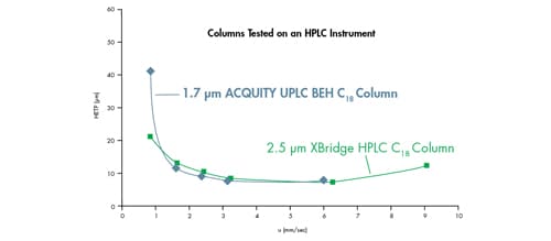
Figure 33: Sub-3 µm particle comparison on an HPLC instrument resulting in similar performance and linear velocity range. van Deemter curves for acenaphthene on an XBridge™ HPLC C18 2.1 x 50 mm, 2.5 µm column and an ACQUITY UPLC BEH C18 2.1 x 50 mm, 1.7 µm column.
The same experiment was then conducted on an ACQUITY UPLC Instrument [band spread = 2.8 µL]. The ACQUITY UPLC Instrument has approximately 84% lower system volume and 60% lower band spreading than the HPLC instrument.
As can be seen in Figure 34, a noticeable difference is observed in the performance of these two columns when operated on the ACQUITY UPLC Instrument. In addition to the observed differences in HETP, the optimal linear velocity increases from 3.0 mm/sec [2.5 µm particle] to 10.0 mm/sec [1.7 µm particle], demonstrating the performance gains of lower HETP [higher efficiency] and faster linear velocity [and therefore throughput] associated with UPLC Technology.
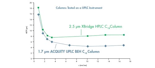
Figure 34: Sub-3 µm particle comparison on an ACQUITY UPLC Instrument resulting in improved performance and linear velocity range with decreasing particle size. van Deemter curves for acenaphthene on an XBridge HPLC C18 2.1 x 50 mm, 2.5 µm column and an ACQUITY UPLC BEH C18 2.1 x 50 mm, 1.7 µm column.
Maintaining Separation Integrity without Compromise
Now that a basic understanding of the functions of extra-column and intra-column band spreading has been established, we can relate the measure of those terms [HETP vs. linear velocity] in a manner that is more practical: plate count vs. flow rate.
As discussed previously, linear velocity is the speed of the mobile phase as it flows through the column. It is a term used to normalize the flow rate of the mobile phase independent of column ID, such that the performance of columns with different dimensions can be measured and compared. The optimal linear velocity is directly related to the optimal flow rate [Figure 35]. Conventional HPLC columns can only be operated in a narrow flow-rate range to achieve the optimum performance. If one operates outside of this range, a decrease in performance can be expected.
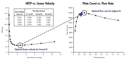
Figure 35: Optimal linear velocity corresponds to optimal flow rate to achieve maximum performance. Values were calculated for a 2.1 mm ID x 50 mm long column packed with 1.7 µm particles.
A common approach to reduce analysis time [improve throughput] in conventional HPLC is to simply increase the flow rate. With larger particles, increasing the flow rate often results in a substantial loss in efficiency, and therefore resolution, since you are now operating above the optimal linear velocity for the HPLC particle [compressed chromatography]. This is a significant compromise between chromatographic performance and analysis speed that is associated with HPLC [Figure 36].
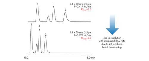
Figure 36: In HPLC, a compromise between resolution and speed must be made. In this case, a 30% loss in resolution is observed.
UPLC Technology is not prone to these compromises. Analysis time can be decreased without sacrificing performance. When particle size is reduced from 3.5 µm to 1.7 µm, a meaningful increase in efficiency is observed [Figure 37]. This is due to the narrow chromatographic bands that are produced by 1.7 µm particle UPLC columns as a result of negligible intra-column band spreading. Additionally, this added efficiency occurs at a higher flow rate [Figure 37]. This means that for the same column length, a dramatic increase in efficiency, and therefore resolution, can be achieved in a shorter analysis time.
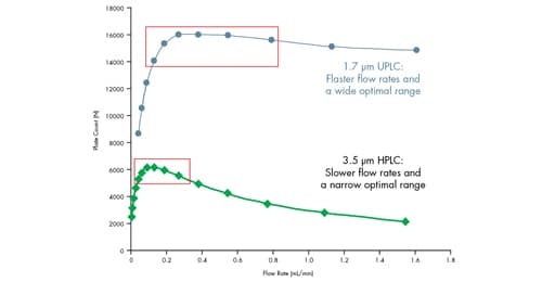
Figure 37: Dependence of particle size on optimal flow rate.
Understanding Column Resolving Power [L/dp]
When performing a chromatographic separation, the primary goal is to resolve one component from another so that some or all of the components can be measured. The maximum resolving power of a column can be estimated by dividing the column length [L] by the particle size [dp]. The L/dp ratio is particularly useful when trying to determine which particle size packing material and column length may be necessary for a given application [Figure 38].
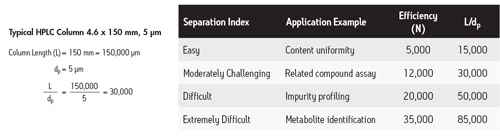
Figure 38: Calculating the L/dp ratio.
This ratio can also be used as a tool for transferring methods from one particle size to another. A column that has an L/dp ratio of 30,000 [moderately challenging separation] is a very common selection. As can be seen in Figure 39, a typical HPLC column that produces a resolving power of 30,000 is 150 mm long and is packed with 5 µm particles. As particle size is decreased, the same resolving power can be achieved in a shorter column [which means faster analysis time; i.e. a 50 mm long column packed with 1.7 µm particles achieves an L/dp ratio of 30,000]. In addition to shorter column length, the optimal flow rate increases as particle size decreases, which further adds to the reduction in analysis time.
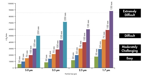
Figure 39: Comparing the L/dp ratio as a function of separation index [easy-to-extremely difficult]. Columns with the same L/dp ratio will generate the same resolving power.
This is more clearly demonstrated chromatographically [Figure 40]. A 50 mm long UPLC column packed with 1.7 µm particles produces the same resolving power as a 150 mm long HPLC column packed with 5 µm particles. By keeping the L/dp ratio constant, analysis time is shortened 10´ while resolution was maintained. Flow rates were adjusted in inverse proportion to each particle size. Injection volumes were scaled in proportion to the column volume such that the same mass load on-column was injected.
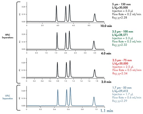
Figure 40: Holding L/dp constant while reducing particle size enables faster separations while maintaining separation integrity.
Understanding the role of column-length-to-particle-size ratio [L/dp] is key to the understanding of UPLC Technology. UPLC Technology is based upon efficiently packing small, pressure-tolerant particles into short [high-throughput] or long [high-resolution] columns. These UPLC columns are used in an LC instrument designed to operate at the optimal linear velocity [and resulting pressure] for these particles with minimal band spreading.
Measuring Gradient Separation Performance [Peak Capacity]
Under isocratic conditions, plate count [N] is a measure of the cumulative band spreading contributions of the instrument and the column. Due to diffusion related band broadening, the width of an analyte band increases the longer the analyte band is retained on the stationary phase.
In a gradient run, the elution strength of the mobile phase changes over the course of the analysis. This causes stronger retained analyte bands to move more quickly through the column [thus changing retention time], keeping the bands more concentrated [narrow]. In reversed-phase chromatography, the increasing elution strength of the mobile phase controls the width of the bands being produced, resulting in similar peak widths as the bands pass through the detector. Since peak width and retention time are being altered by the changing strength of mobile phase, plate count [due to its relationship to peak width] is not a valid measurement for gradient separations.
The resolving [separation] power of a gradient can be calculated by its peak capacity [Pc]. Thus, peak capacity is simply the theoretical number of peaks that can be separated in a given gradient time. Peak capacity is inversely proportional to peak width. Therefore, for Pc to increase, peak width must decrease.

Figure 41: Peak capacity [Pc] equation, where [tg] is the gradient time and [w] is the average peak width.
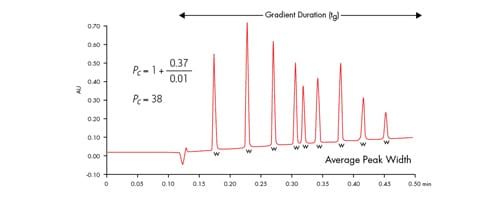
Figure 42: Applying the peak capacity equation to a fast separation, where 0.37 minutes is the gradient duration time and 0.01 minutes is the average peak width, resulting in a peak capacity of 38. Peak width was measured at 13.4% peak height [4σ].
Peak capacity can be dramatically increased by using UPLC Technology. The high resolving power of UPLC Technology enables more information per unit time to be generated by harnessing the power of sub-2 µm particles on exceptionally low dispersion instrumentation [2.8 µL band spread]. This facilitates more information that can be collected from a given sample. For example, a tryptic digest of phosphorylase b yields ~70 identified peaks using an HPLC column packed with 5 µm particles [Figure 43A]. With UPLC Technology, the number of identifiable peaks increases from 70 to 168, thus improving confidence in protein identification [Figure 43B].
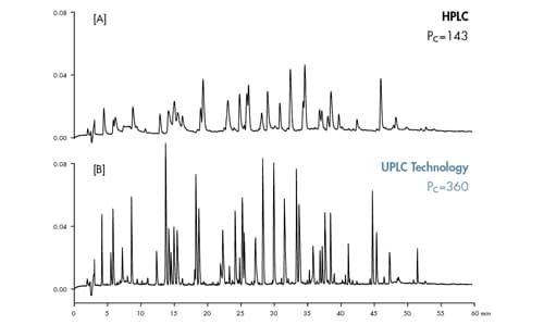
Figure 43: Peak capacity comparison of HPLC vs. UPLC Technology.